Week 3.5 - Deriving 4th order approximation of a 2nd order derivative using Taylor Table method

AIM :

To write a program in Matlab to evaluate the second-order derivative of the analytical function exp(x)*cos(x) and compare it with the 3 numerical approximations that's been derived.

THEORY :

Discretization : Discretization is the process of transferring continuous functions, models, variables, and equations into discrete counterparts. This process is usually carried out as a first step toward making them suitable for numerical evaluation and implementation on digital computers. Discretization can be used in deducing and translating any Nth order continuous differential derivative into discrete ordinary differential equations. We primarily discretize them based on three different techniques to achieve the most efficient results.

• Central Difference Technique : It is a method where values are obtained symmetrically from the central main node to get accurate derivative.For instance, if i want to calculate the 4th order Accuracy requried for second-order derivative i need the computed resultant of 2 nodes from both sides: i-2,i-1,i,i+1,i+2, which is 5 nodal values including the main node solving for the corresponding derivative function.

The order of accuracy P = Number of nodes in the stencil N - order of derivative Q + 1 for symmetric/central schemes

P = N - Q + 1 -------- (1)

• Right Skewed Difference Technique : It is a method where values are obtained from the right / positive coordinate values / Forward from the central main node to get accurate derivative.For instance, if i want to calculate 4th order Accuracy requried for second-order derivative i need the computed resultant of 4 nodes from central to right side: i,i+1,i+2,i+3,i,i+4,i+5, which is 6 nodal values including the main node solving for the corresponding derivative function.

The order of accuracy P = Number of nodes in the stencil N - order of derivative Q for one-sided/skewed schemes

P = N - Q --------- (2)

• Left Skewed Difference Technique : It is a method where values are obtained from the left / negative coordinate values / Backward from the central main node to get accurate derivative.For instance, if i want to calculate 4th order Accuracy requried for second-order derivative i need the computed resultant of 4 nodes from central to right side: i,i-1,i-2,i-3,i,i-4,i-5, which is 6 nodal values including the main node solving for the corresponding derivative function.

The order of accuracy P = Number of nodes in the stencil N - order of derivative Q for one-sided/skewed schemes

P = N - Q --------- (2)

Truncation Error : Truncation is a method of approximating numbers. It is easier than rounding, but does not always
give the best approximation to the original number. Truncation is used in computing when division
is done with integers and the answer must be an integer.

Rounding Error : A rounding error is the difference between the result produced by a given algorithm using exact arithmetic and the result produced by the same algorithm using finite-precision, rounded arithmetic.Rounding errors are due to inexactness in the representation of real numbers and the arithmetic operations done with them.

One of the goals of numerical analysis is to estimate computation errors.Computation errors, also called numerical errors, include both truncation erros and roundoff errors.

So from understanding the skewed & symmetrical differences, we see that forward / backward difference schemes fall under the skewed and central differencing falls under the symmetric difference.

clear all
close all
clc

x = pi/3;
dx = linspace(pi/40,pi/4000,20);


% for i = 1 : length(dx)
% [skewed_left_error(i),skewed_right_error(i),central_diff_error(i),skewed_left(i),skewed_right(i),central_diff(i)] = second_deriv(x,dx) 
% end

f = @(x) exp(x).*cos(x);

analytical = -2*exp(x)*sin(x); % analytical derivative 

%Central_differencing
A = [1,1,1,1,1;-2,-1,0,1,2;4,1,0,1,4;-8,-1,0,1,8;16,1,0,1,16];
B = [0;0;2;0;0];
X = inv(A)*B;
 
%hypothesis function
C_D = (X(1)*f(x-2*dx) + X(2)*f(x-dx) + X(3)*f(x) + X(4)*f(x+dx) + X(5)*f(x+2*dx))./dx.^2;
er_cd = abs((C_D - analytical));

%Right_Skewed_Scheme
C = [1,1,1,1,1,1;0,1,2,3,4,5;0,1,4,9,16,25;0,1,8,27,64,125;0,1,16,81,256,625;0,1,32,243,1024,3125];
D = [0;0;2;0;0;0];
Y = inv(C)*D;

S_R = (Y(1)*f(x) + Y(2)*f(x+dx) + Y(3)*f(x+2*dx) + Y(4)*f(x+3*dx) + Y(5)*f(x+4*dx) + Y(6)*f(x+5*dx))./dx.^2;
er_sr = abs((S_R - analytical));

%Left Skewed Scheme
L = [1,1,1,1,1,1;0,-1,-2,-3,-4,-5;0,1,4,9,16,25;0,-1,-8,-27,-64,-125;0,1,16,81,256,625;0,-1,-32,-243,-1024,-3125];
M = [0;0;2;0;0;0];
N = inv(L)*M;


S_L = (N(1)*f(x) + N(2)*f(x-dx) + N(3)*f(x-2*dx) + N(4)*f(x-3*dx) + N(5)*f(x-4*dx) + N(6)*f(x-5*dx))./dx.^2;
er_sl = abs((S_L - analytical));

loglog(dx,er_cd,dx,er_sr,dx,er_sl)
xlabel("Grid Size")
ylabel("Error")
title("Error Comparison for different schemes using Taylor Table")
legend('Symmetric Scheme','Right Skewed Scheme','Left Skewed Scheme')

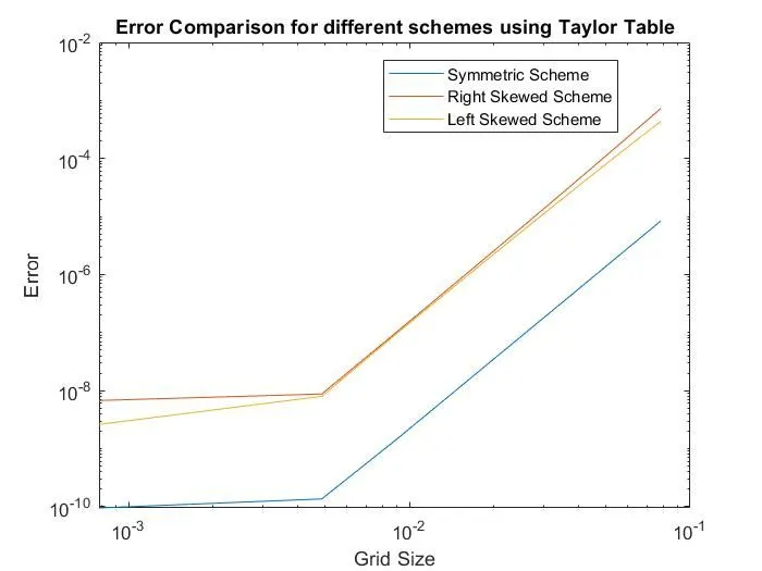
CODE :

• First we intialize the main node, which is x = pi/ 3 is the main nodal point from which we are going to calculate the next nodal point based on the finite difference methods.
• Next we have the step sizes from grid to grid fixed, this is specified using the linspace command of 'dx'.
• Now we initialize a variable 'f', inside which we specify the inline function and variable 'x'.
• To calculate the exact / accurate solution to weigh aganist the numerical method resultants , we need to find the analytical value of the function.
• Let us calculate the double derivative of `e^x cos x`.
• Now to calculate the double derivative of the above function we need to apply the differential law.

`(e^x)*(-sin x) + (cos x) e^x + (e^x)*(-sin x) + (cos x) e^x`

`(e^x)*(-sin x) + (e^x)*(-sin x)`

`-2.e^x sin x`

• Using the taylor's table method, we shall find the linear equations based on the corresponding order of approximation and the derivative to be solved to ordinary differential equation.
• Now once we obtain the coefficients for the linear equations, we insert the coefficients inside the 'A' Matrix & the B matrix has the unknowns , and the only the derivative function we are solving for , has a value of 2. This is because when we substitute the formulae to solve for the corresponding derivative in the taylor's table, we obtain the value as a constant.
• As we know the formulae, `X = A^-1*B`, Here X - Resultant Matrix / Matrix of Unknowns we need to solve for.
• We compute the values for all the three difference methods in a similar fashion.
• From which we deduce the equation for Hypothesis function.
• Finally, we calculate the absolute error , by differencing the actual value from the numerically calculate value.

Inference :

• We can observe that all the three difference plots are sid to have a similar slope and not a great deviation.
• As dx increases, the error is said to increase propotionately for both right skewed and left skewed compared to central / symmetric difference method.
• Symmetric Differene is said to posit a lesser error figure compared to ts counterparts. An error factor of `10^-2`.
• Skewed Difference is comparatively preferable if in the case where we are expected to calculate the values from a specific boundary condition.
• We can also notice that, as the dx / grid size plummets, we can see that there is a deviation from the actual graphical plot, this gives rise to slope and also introduction to truncation and round off error which causes major instability and inconsistency in the results obtained