Challenge

Week 8 - Simulation of a backward facing step in OpenFOAM

AAkash Yadav2 Jun 2022

Laminar Flow over a Backward Facing Step:

Fluid seperation his a common and interesting. Thus it has been an area of intensive study for many years. Some classical applications includes -a flow in a pipe with sudden expanion, flow in a pipe with an obstruction, flow in a channel with an obstruction and flow in a channel with sudden expansion.

Among these, the backward-facing step flow has become a very popular benchmarking and validation test for computational fluid dynamics (CFD) simulations owing to its simple geomety and the availability of a good number of quality experimental data.

The flow is divided into 7 regions:

Region I: Initial Boundary Layer.
The flow extends from entry point of the geometry to the step inside the geometry.
Region II: Seperated Free Shear Layer.
The flow seperates from the wall and results in a free shear layer. The state of initial boundary layer is the main parameter that affects the development of free shear layer. This unstable free shear layer then splits into 2 parts. A part goes in reattachment zone (region III) while a significant part of the flow is reversed upstream and goes on to supply the recirculation stream (region IV).
Region III: Reattachment Zone.
The seperated free shear layer reattaches with the bottom face while the rest goes in recirculation region.
Region IV: Primary Recirculation Layer.
This region of the flow is characterized by the recirculating vortices and flow reversal. Maximum backflow velocity are reported to be around 20% of the mean bulk flow from experimental measurements. The backflow reamins strongly viscous dominated.
Region V: Corner Eddy.
Region VI: Redeveloping Boundary Layer.
The flow after reattachment with lower face starts developing again.
Region V: Second Seperation Region.
Depending on the reynolds number based on step height (`Re_h`) of the flow there may or may not be a secondary seperation zone. The secondary seperation region starts to increase for `Re_h`>300 and gradually decreases afterwards until it completely diminishes for `Re_h`=4950. This seperation region is attributed to adverse pressure gradient associated with sudden change in cross section of the channel.

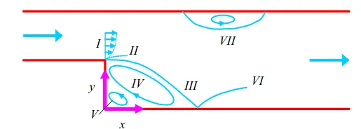
We are required to create the following geometry by copying a case study from tutorials directory of OpenFOAM and modifying the blockMeshDict file.

Then we have to simulate the flow through the geometry using:

Uniform cell size.
Non uniform cell size using simplegrading.

and compare the results from both the simulations.

1) We first begin with going to the tutorials directory and copy a case file to OpenFoam-run directory. This is done as the changes made in the tutorial directory are irreversible and to get the original files one may have to install the openFoam package again. Following commands are carried out in the terminal to achieve this:

tut
cd incompressible/icoFoam/
cp -r cavity/ $FOAM_RUN/cavity_test
cd $FOAM_RUN/cavity_test/
gedit system/blockMeshDict

The blockMeshDict file looks like this:

/*--------------------------------*- C++ -*----------------------------------*\
  =========                 |
  \\      /  F ield         | OpenFOAM: The Open Source CFD Toolbox
   \\    /   O peration     | Website:  https://openfoam.org
    \\  /    A nd           | Version:  9
     \\/     M anipulation  |
\*---------------------------------------------------------------------------*/
FoamFile
{
    version     2.0;
    format      ascii;
    class       dictionary;
    object      blockMeshDict;
}
// * * * * * * * * * * * * * * * * * * * * * * * * * * * * * * * * * * * * * //

convertToMeters 1;

vertices
(
    (0 0 0)            //0
    (0.08 0 0)         //1
    (0.08 0.005 0)     //2
    (0 0.005 0)        //3
    (0.08 0.01 0)      //4
    (0 0.01 0)         //5
    (0.20 0.01 0)      //6
    (0.20 0.005 0)     //7
    (0.20 0 0)         //8
    (0.20 -0.01 0)     //9
    (0.08 -0.01 0)    //10
    (0 0 0.1)         //11
    (0.08 0 0.1)      //12
    (0.08 0.005 0.1)  //13
    (0 0.005 0.1)     //14
    (0.08 0.01 0.1)   //15
    (0 0.01 0.1)      //16
    (0.20 0.01 0.1)   //17
    (0.20 0.005 0.1)  //18
    (0.20 0 0.1)      //19
    (0.20 -0.01 0.1)  //20
    (0.08 -0.01 0.1)  //21
);

blocks
(
    hex (0 1 2 3 11 12 13 14) (80 5 1) simpleGrading (1 1 1)  //Block1
    hex (3 2 4 5 14 13 15 16) (80 5 1) simpleGrading (1 1 1) //Block2
    hex (2 7 6 4 13 18 17 15) (120 5 1) simpleGrading (1 1 1) //Block3
    hex (1 8 7 2 12 19 18 13) (120 5 1) simpleGrading (1 1 1)  //Block4
    hex (10 9 8 1 21 20 19 12) (120 10 1) simpleGrading (1 1 1) //Block5
);

edges
(
);

boundary
(
    inlet
    {
        type patch;
        faces
        (
            (0 11 14 3)
            (3 14 16 5)
        );
    }
    outlet
    {
        type patch;
        faces
        (
            (9 8 19 20)
            (8 7 18 19)
            (7 6 17 18)
        );
    }
    NoSlipWall
    {
        type wall;
        faces
        (
            (4 5 16 15)
            (4 15 17 6)
            (0 1 12 11)
            (9 20 21 10)
            (1 10 21 12)
        );
    }
    frontAndBack
    {
        type empty;
        faces
        (
            (0 3 2 1)
            (11 12 13 14)
            (3 5 4 2)
            (13 15 16 14)
            (2 4 6 7)
            (13 18 17 15)
            (1 2 7 8)
            (12 19 18 13)
            (10 1 8 9)
            (21 20 19 12) 
        );
    }
);

mergePatchPairs
(

);



(
);
// ************************************************************************* //

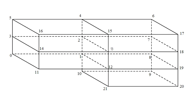
We have subdivided our geometry into 5 smaller geometries. Each of these smaller geometry is defined using vertices of the respective geometry under the title 'blocks'.

We also see simpleGrading afer defining number of cells for each smaller geometries. Often its desirable to study a phenomena occuring in a particular part of the domain. To capture that phenomen perfectly, its desirable to have a much finer mesh. While this is an obvious way to go,going for a finer mesh also increases the computational effort and simulation time drastically. What can be done about this is to have fine mesh where necessary while having a coarser mesh structure elsewhere. This is exactly what simpleGrading is use for. It is used to create non-uniform mesh across the geometry along x,y & directions.

Format for simpleGrading is "simpleGrading (`n_x` `n_y` `n_z`) where `n_x` , `n_y` & `n_z` represent the ratio of length of final and intial cell along x, y and z directions respectively.

For non-uniform grid spacing, following changes are made in the 'simpleGrading' values under block section of blockMeshDict file of the case study.

blocks
(
    hex (0 1 2 3 11 12 13 14) (80 5 1) simpleGrading (0.2 20 1)  //Block1
    hex (3 2 4 5 14 13 15 16) (80 5 1) simpleGrading (0.2 0.2 1) //Block2
    hex (2 7 6 4 13 18 17 15) (120 5 1) simpleGrading (20 0.2 1) //Block3
    hex (1 8 7 2 12 19 18 13) (120 5 1) simpleGrading (20 20 1)  //Block4
    hex (10 9 8 1 21 20 19 12) (120 10 1) simpleGrading (20 20 1) //Block5
);

The geometry and mesh for both the cases are shown below:

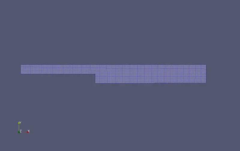
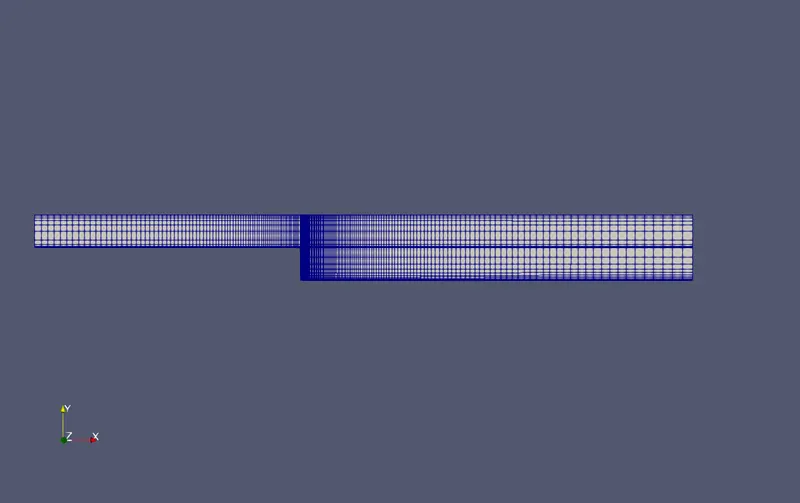
2) We go to '0' directory and make changes to 'p' and 'U' FOAM files. We change the default boundary conditions with our own depending upon the geometry.

/*--------------------------------*- C++ -*----------------------------------*\
  =========                 |
  \\      /  F ield         | OpenFOAM: The Open Source CFD Toolbox
   \\    /   O peration     | Website:  https://openfoam.org
    \\  /    A nd           | Version:  9
     \\/     M anipulation  |
\*---------------------------------------------------------------------------*/
FoamFile
{ 
    version     2.0;
    format      ascii;
    class       volScalarField;
    object      p;
}
// * * * * * * * * * * * * * * * * * * * * * * * * * * * * * * * * * * * * * //

dimensions      [0 2 -2 0 0 0 0];

internalField   uniform 0;

boundaryField
{
    inlet
    {
        type            zeroGradient;
    }

    outlet
    {
        type            fixedValue;
        value           uniform 0;
    }

    NoSlipWall
    {
        type            zeroGradient;
    }

    frontAndBack
    {
        type            empty;
    }
}

// ************************************************************************* //

/*--------------------------------*- C++ -*----------------------------------*\
  =========                 |
  \\      /  F ield         | OpenFOAM: The Open Source CFD Toolbox
   \\    /   O peration     | Website:  https://openfoam.org
    \\  /    A nd           | Version:  9
     \\/     M anipulation  |
\*---------------------------------------------------------------------------*/
FoamFile
{
    version     2.0;
    format      ascii;
    class       volVectorField;
    object      U;
}
// * * * * * * * * * * * * * * * * * * * * * * * * * * * * * * * * * * * * * //

dimensions      [0 1 -1 0 0 0 0];

internalField   uniform (0 0 0);

boundaryField
{
    inlet
    {
        type            fixedValue;
        value           uniform (0.1 0 0);
    }

    outlet
    {
        type            zeroGradient;
    }

    NoSlipWall
    {
        type            noSlip;
    }

    frontAndBack
    {
        type            empty;
    }
}

// ************************************************************************* //

3) We make changes in 'endTime' and 'deltaT' values in controlDict file, in system directory of case directory, so that our courant number remains below 1 and our solution doesn't blow.

/*--------------------------------*- C++ -*----------------------------------*\
  =========                 |
  \\      /  F ield         | OpenFOAM: The Open Source CFD Toolbox
   \\    /   O peration     | Website:  https://openfoam.org
    \\  /    A nd           | Version:  9
     \\/     M anipulation  |
\*---------------------------------------------------------------------------*/
FoamFile
{
    version     2.0;
    format      ascii;
    class       dictionary;
    location    "system";
    object      controlDict;
}
// * * * * * * * * * * * * * * * * * * * * * * * * * * * * * * * * * * * * * //

application     icoFoam;

startFrom       startTime;

startTime       0;

stopAt          endTime;

endTime         3;

deltaT          1e-4;

writeControl    timeStep;

writeInterval   50;

purgeWrite      0;

writeFormat     ascii;

writePrecision  6;

writeCompression off;

timeFormat      general;

timePrecision   6;

runTimeModifiable true;


// ************************************************************************* //

4) Running blockMesh to generate the mesh followed by icoFoam to solve and obtain the solution. icoFoam is the solver we have used. It is a transient laminar incompressible solver which solves the problem transiently until steady state is achieved.

5) Running paraFoam to run the simulation and display the results.

Results:

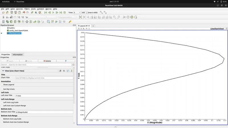
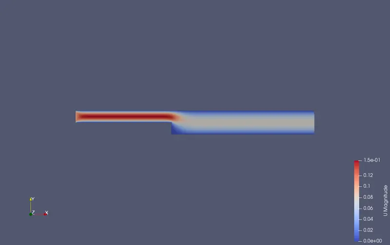
The following plots were obtained for both the cases:

1)Uniform Mesh

2) Non-uniform mesh

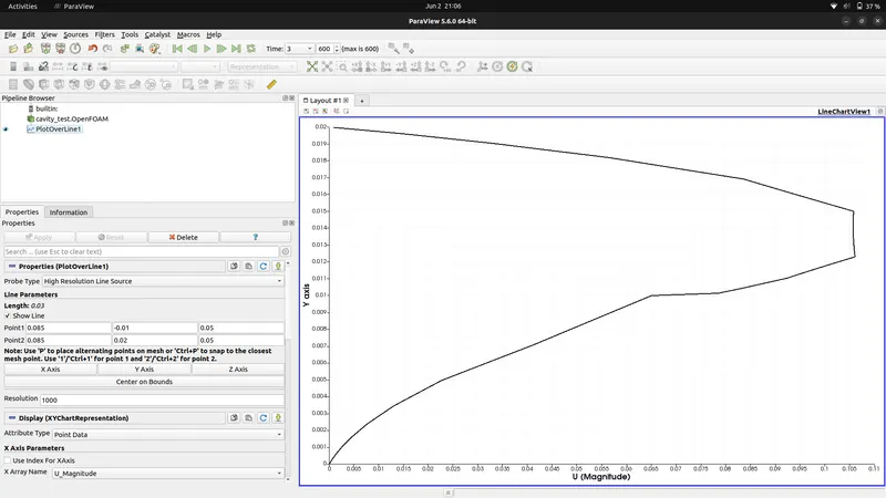
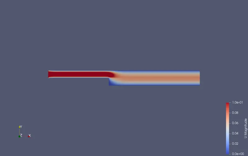
We observe from the above plots we see the second plot is much more detailed and velocity profile is more pronounced. Also, the second velocity profile is much more consistent with the actual velocity profile than the first one.

The velocity profile at 0.085 m from inlet is shown above with uniform and non-uniform grid spacing. we find the plot for uniform grid spacing is more similar to flow between parallel plates and doesnt capture the flow seperation properly as the case with non-uniform grid spacing does.

Conclusion:

Finer the mesh, more accurate are the results.
Mesh should be refined in areas where we want to capture the flow more accurately to reduce the computational efforts and reduce the simulation time.

References:

Week 8 - Simulation of a backward facing step in OpenFOAM

Ship work like this
in your own course.

Talk to a career counsellor

Ship work like thisin your own course.

Talk to a career counsellor

Ship work like this
in your own course.

References:

- https://www.researchgate.net/profile/Carlo-Gualtieri/publication/240157000_Numerical_Simulations_of_Laminar_Backward-Facing_Step_Flow_With_FEMLAB_31/links/00b7d5253f4010cb68000000/Numerical-Simulations-of-Laminar-Backward-Facing-Step-Flow-With-FEMLAB-31.pdf?origin=publication_detail
- https://cfd-training.com/2019/04/06/backward-facing-step-laminar-flow/