Week 8 - Simulation of a backward facing step in OpenFOAM
Objective :
- Use OpenFOAM to simulate the fluid flow in a backward-facing step.
- Edit the blockMeshDict, controlDict, U, P file to solve the required problem.
- Study effect of grading factor in simulation.
OpenFoam has many tutorial folders that can be used and edited to simulate the specific problem user wants.
Here, we will try to simulate laminar, incompressible viscous flow through a duct which is given below,
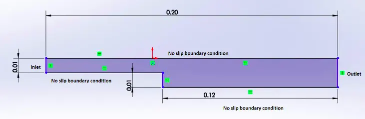
Although the flow will be two-dimensional, the duct has a thickness in the direction perpendicular to the paper, but that does not affect the flow, and the flow field is two-dimensional. The inlet is at left, outlet at right, top and bottom face are walls, the middle step is a wall too.
cavityTo start the simulation, we need to copy the cavity folder from $FOAM_TUTORIALS/incompressible/icoFoam/cavity/cavity to $FOAM_RUN.
After copying, go to $FOAM_RUN/cavity, where now will find folder 0, constant, system.
Step 1 :
To simulate the flow through backward step duct, we will divide the domain into block's of cuboid as shown below,
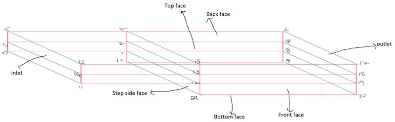
There is a total of 5 blocks, each defined by vertices as shown. The coordinate system origin is at vertex '0', where +ve x-axis is along edge '0-1', +ve y-axis along edge '0-11', and z-axis following right hand rule. This is important because while coding each block, one should always input vertices such that when one sees the face of the block in front, the outward normal should point towards oneself.
The code to edit is in the system folder named as blockMeshDict.
*--------------------------------*- C++ -*----------------------------------*\
  =========                 |
  \\      /  F ield         | OpenFOAM: The Open Source CFD Toolbox
   \\    /   O peration     | Website:  https://openfoam.org
    \\  /    A nd           | Version:  9
     \\/     M anipulation  |
\*---------------------------------------------------------------------------*/
FoamFile
{
    format      ascii;
    class       dictionary;
    object      blockMeshDict;
}
// * * * * * * * * * * * * * * * * * * * * * * * * * * * * * * * * * * * * * //

convertToMeters 0.01;

vertices
(
    (0 0 0) // 0
    (8 0 0) // 1
    (8 0.5 0) // 2
    (0 0.5 0) // 3
    (8 1 0) // 4
    (0 1 0) // 5
    (20 1 0) // 6
    (20 0.5 0) //7
    (20 0 0) // 8
    (20 -1 0) // 9
    (8 -1 0) // 10
    (0 0 0.1) // 11
    (8 0 0.1) // 12
    (8 0.5 0.1) // 13
    (0 0.5 0.1) // 14
    (8 1 0.1) // 15
    (0 1 0.1) //16
    (20 1 0.1) //17
    (20 0.5 0.1) // 18
    (20 0 0.1) // 19
    (20 -1 0.1) // 20
    (8 -1 0.1) // 21
);

blocks
(
    // For gradind factor 0.2
    /*
    hex (0 1 2 3 11 12 13 14) (80 5 1) simpleGrading (0.2 5 1) // block 1
    hex (3 2 4 5 14 13 15 16) (80 5 1) simpleGrading (0.2 0.2 1) // block 2
    hex (10 9 8 1 21 20 19 12) (120 10 1) simpleGrading (5 5 1) // block 3
    hex (1 8 7 2 12 19 18 13) (120 5 1) simpleGrading (5 5 1) // block 4
    hex (2 7 6 4 13 18 17 15) (120 5 1) simpleGrading (5 0.2 1) // block 5
    */

    // For gradind factor 1

    hex (0 1 2 3 11 12 13 14) (80 5 1) simpleGrading (1 1 1) // block 1
    hex (3 2 4 5 14 13 15 16) (80 5 1) simpleGrading (1 1 1) // block 2
    hex (10 9 8 1 21 20 19 12) (120 10 1) simpleGrading (1 1 1) // block 3
    hex (1 8 7 2 12 19 18 13) (120 5 1) simpleGrading (1 1 1) // block 4
    hex (2 7 6 4 13 18 17 15) (120 5 1) simpleGrading (1 1 1) // block 5

);

edges
(
);

boundary
(
    inlet
    {
        type patch;
        faces
        (
            (0 11 14 3)
            (3 14 16 5)
        );
    }
    outlet
    {
        type patch;
        faces
        (
            (6 17 18 7)
            (7 18 19 8)
            (8 19 20 9)
        );
    }
    frontAndBack
    {
        type empty;
        faces
        (
            (0 3 2 1)
            (3 5 4 2)
            (10 1 8 9)
            (1 2 7 8)
            (2 4 6 7)
            (16 14 13 15)
            (14 11 12 13)
            (15 13 18 17)
            (13 12 19 18)
            (12 21 20 19)
        );
    }
    upperwalls
    {
     	type wall;
     	faces
     	(
     	     (16 15 4 5)
     	     (15 17 6 4)
     	);
     }
     lowerwalls
     {
     	type wall;
     	faces
     	(
     	     (11 0 1 12)
     	     (21 10 9 20)
     	     (1 10 21 12)
     	);
     }
);

mergePatchPairs
(
);

// ************************************************************************* //
First define all the vertex (x, y, z) in vertices block. After defining all the vertex, go to blocks section, where define all 5 blocks using the vertices. hex ( 0 1 2 3 11 12 13 14) defines the first block. After that (nx , ny, nz) defines the number of cells in the x, y, z directions respectively. Since the flow is 2-d, one cell in the z-direction is fine.simpleGrading (x_value, y_value, z_value) sets the grading factor in x, y, z-direction respectively.
Similarly, repeat the process for other blocks.
Grading factor = (size of end cell)/(size of start cell). A simple grading of less than 1 means end cell size is less than start cells and so the end side is more refined and vice versa. A grading factor of 1 means uniform cells throughout the domain. This is useful because cell refinement helps improve and get better results, especially around boundary layers.
Once all blocks are defined go to boundary section to define the boundary of the domain. For each boundary, one needs to provide the type and faces of the boundary. For example, for inlet boundary, the type is a patch, since made of two blocks and faces, are (0 11 14 3), (3 14 16 5). Type wall is used for faces that act as walls (no-slip) i.e. top, bottom, and side faces, type empty is used for faces that are part of dimension which is not active in simulation i.e. front and back faces.
Once all this is done save the code.
Step 2 :
Go to controlDict code which is in same folder.
/*--------------------------------*- C++ -*----------------------------------*\
  =========                 |
  \\      /  F ield         | OpenFOAM: The Open Source CFD Toolbox
   \\    /   O peration     | Website:  https://openfoam.org
    \\  /    A nd           | Version:  9
     \\/     M anipulation  |
\*---------------------------------------------------------------------------*/
FoamFile
{
    format      ascii;
    class       dictionary;
    location    "system";
    object      controlDict;
}
// * * * * * * * * * * * * * * * * * * * * * * * * * * * * * * * * * * * * * //

application     icoFoam;

startFrom       startTime;

startTime       0;

stopAt          endTime;

endTime         0.5;

deltaT          0.0001;

writeControl    timeStep;

writeInterval   50;

purgeWrite      0;

writeFormat     ascii;

writePrecision  6;

writeCompression off;

timeFormat      general;

timePrecision   6;

runTimeModifiable true;


// ************************************************************************* //
Here, define the startTime (0) , endTime (0.5) , deltaT (0.0001) and writeInterval (50).
deltaT value is the time interval or time step the user defines. It should be defined such that CFL condition is maintained at all time steps.
CFL = `(|U|deltat)/(deltax) < 1`. If CFL condition is violated, simulation gives an error and it stops at that time step.
writeInterval value defines the time steps at which the solution is stored.
Step 3 :
Go to the constant folder where one needs to set the transport properties in code transportProperties.
/*--------------------------------*- C++ -*----------------------------------*\
  =========                 |
  \\      /  F ield         | OpenFOAM: The Open Source CFD Toolbox
   \\    /   O peration     | Website:  https://openfoam.org
    \\  /    A nd           | Version:  9
     \\/     M anipulation  |
\*---------------------------------------------------------------------------*/
FoamFile
{
    format      ascii;
    class       dictionary;
    location    "constant";
    object      transportProperties;
}
// * * * * * * * * * * * * * * * * * * * * * * * * * * * * * * * * * * * * * //

nu              [0 2 -1 0 0 0 0] 1e-5;


// ************************************************************************* //
Define the nu value (kinematic viscosity) as 1e-5 so that the Reynolds number is such that flow is laminar.
Step 4 :
Go to the folder named '0'. Here, one needs to define boundary conditions value based on boundary type defined in blockMeshDict.
For velocity, the code is :
/*--------------------------------*- C++ -*----------------------------------*\
  =========                 |
  \\      /  F ield         | OpenFOAM: The Open Source CFD Toolbox
   \\    /   O peration     | Website:  https://openfoam.org
    \\  /    A nd           | Version:  9
     \\/     M anipulation  |
\*---------------------------------------------------------------------------*/
FoamFile
{
    format      ascii;
    class       volVectorField;
    object      U;
}
// * * * * * * * * * * * * * * * * * * * * * * * * * * * * * * * * * * * * * //

dimensions      [0 1 -1 0 0 0 0];

internalField   uniform (0 0 0);

boundaryField
{
    inlet
    {
        type            fixedValue;
        value           uniform (1 0 0);
    }

    outlet
    {
        type            zeroGradient;
    }

    upperwalls
    {
        type            noSlip;
    }

    lowerwalls
    {
        type            noSlip;
    }

    frontAndBack
    {
        type            empty;
    }
}

// ************************************************************************* //
dimensions [0 1 -1 0 0 0 0] define the dimension of flow field. The first digit is for mass, the second for length, and the third for time. Other digits are for other fundamental dimensions. For velocity, it is m/s.
internalField is defined as uniform with value (0 0 0 ) representing velocity in x, y, z-direction respectively.
boundaryField for each boundary should have information about type and value. For inlet, type is fixed value of (1 0 0). For outlet, one floats the value as zero gradient. The Top, bottom, and sidestep face is of the type no slip. Front and back faces are of type empty.
For pressure, the code is :
/*--------------------------------*- C++ -*----------------------------------*\
  =========                 |
  \\      /  F ield         | OpenFOAM: The Open Source CFD Toolbox
   \\    /   O peration     | Website:  https://openfoam.org
    \\  /    A nd           | Version:  9
     \\/     M anipulation  |
\*---------------------------------------------------------------------------*/
FoamFile
{
    format      ascii;
    class       volScalarField;
    object      p;
}
// * * * * * * * * * * * * * * * * * * * * * * * * * * * * * * * * * * * * * //

dimensions      [0 2 -2 0 0 0 0];

internalField   uniform 0;

boundaryField
{
    inlet
    {
        type            zeroGradient;
    }

    outlet
    {
        type            fixedValue;
        value		 uniform 0;
    }

    upperwalls
    {
        type            zeroGradient;
    }

    lowerwalls
    {
        type            zeroGradient;
    }

    frontAndBack
    {
        type            empty;
    }
}

// ************************************************************************* //
Here the steps are the same as for velocity. The dimension for pressure is `m^2/s^2`. For inlet, we float the value as zero gradient. At the outlet, the value is fixed as 0. The Top, bottom, sidestep face has zero gradient floated value. The front and back faces are empty.
The folder '0' is the initial conditions folder also.
Step 5 :
Generate the grid by running blockMesh in the terminal. It gives polymesh folder in the constant folder which contains the mesh generated from blockMeshDict code. Once this is done, one can run the code simply by running 'icoFoam' command in the terminal. One should be able to see something like this in the terminal for each time step:
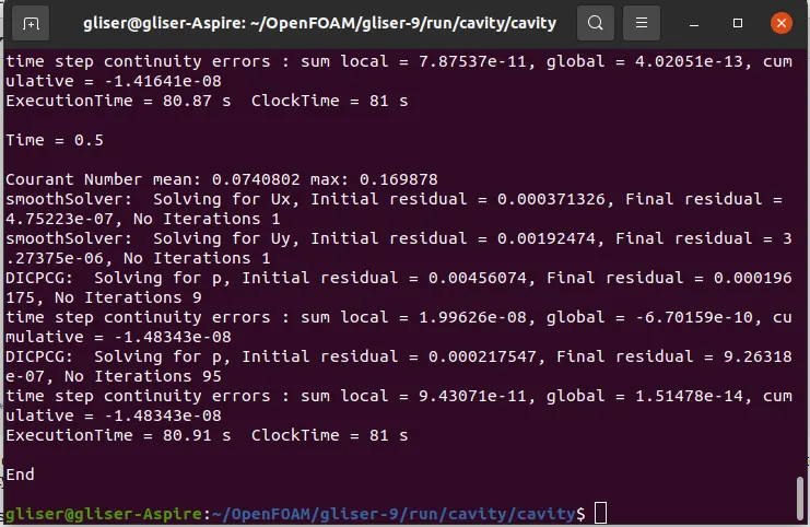
This is detailed information on courant number, residuals, error, execution time, etc.
One will also find a new folder named after the time value. These folder contains the solution at that time. One can easily view the solution by running 'paraFoam' in the terminal, where parafoam gets opened.
OUTPUT :
Case 1 : Grading factor = 1.

The above figure shows the mesh (discretize domain). The mesh is uniform in all dimensions. In the blocks section of blockMeshDict code, set simpleGrading as (1 1 1) for all blocks.
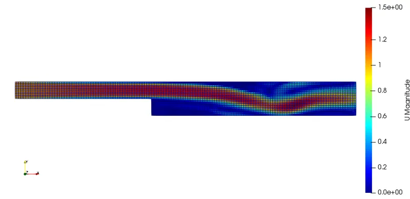
The above figure shows the velocity field inside the domain at time = 0.5 sec. In the section before the step, we can see the boundary layer developed.
Case 2 : Grading factor = 0.2

In blocks section of blockMeshDict code, make changes as follows :
hex (0 1 2 3 11 12 13 14) (80 5 1) simpleGrading (0.2 5 1) // block 1
hex (3 2 4 5 14 13 15 16) (80 5 1) simpleGrading (0.2 0.2 1) // block 2
hex (10 9 8 1 21 20 19 12) (120 10 1) simpleGrading (5 5 1) // block 3
hex (1 8 7 2 12 19 18 13) (120 5 1) simpleGrading (5 5 1) // block 4
hex (2 7 6 4 13 18 17 15) (120 5 1) simpleGrading (5 0.2 1) // block 5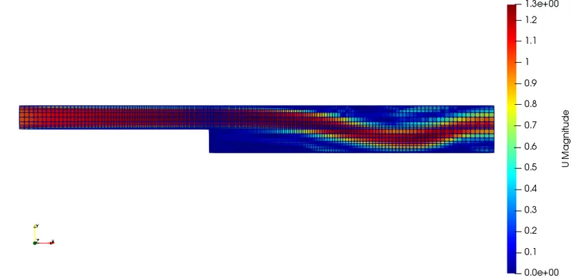
The above figure shows the velocity field inside the domain at time = 0.5 sec. In the section before the step, we can see the boundary layer developed.
Comparison :
1.
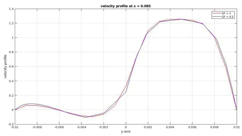
For both grading factor, the velocity profile at x = 0.085 is very close to each other. But we can clearly see close to walls ( y = - 0.01 , y `~~`0, y = 0.01), the profile for grading factor 0.2 is more refined than gf = 1. This is due to more cells near the walls and step. However, since the total number of cells were fixed for both case, this has resulted in less cell in middle for gf = 0.2 than gf = 1. As a result, the profile for gf = 1 is more refined in middle than gf = 0.2.
If one is interested in capturing the boundary layers, more cells are needed close to walls. Thus grading factor help one to do so. GF < 1 close to walls, helps in better resolution of boundary layers.
2.
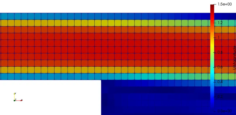
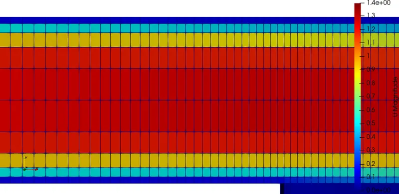
The left figure is for gf = 1 and right one is for gf = 0.2. As can be seen for gf = 0.2, the boundary layer is better captured by more cells close to walls than gf = 1.
Grading factor is important for refinement of cells in the region where one wants to capture some important physical phenomenon.