Week 3.5 - Deriving 4th order approximation of a 2nd order derivative using Taylor Table method

Derivation: This section deals with the derivation of fourth-order approximation of second derivative using central difference, skewed right side difference, and skewed left side difference. To derive the form we will make use of the Taylor table. The derivation is as follows:

1. Central difference : To derive fourth-order taylor approximation of second derivative of f(x) we need a stencil of 5 points, 2 on right side of `f_i` and 2 on left side of `f_i`. Let the general form of approximation be : `(d^2f(x))/(dx^2) approx (delta^2f(x))/(deltax^2)=a*f_(i-2)+b*f_(i-1)+c*f_i+d*f_(i+1)+e*f_(i+2)`. To compute values of a,b,c,d,e, we use Taylor table

   `(delta^2f(x))/(deltax^2)`	`f(x)`	`f^'(x)Deltax`	`f^('')(x)(Deltax^2)/(2!)`	`f^(''')(x)(Deltax^3)/(3!)`	`f^(4)(x)(Deltax^4)/(4!)`	`f^(5)(x)(Deltax^5)/(5!)`	`f^(6)(x)(Deltax^6)/(6!)`
   `a*f_(i-2)`	`a`	`-2*a`	`4*a`	`-8*a`	`16*a`	`-32*a`	`64*a`
   `b*f_(i-1)`	`b`	`-b`	`b`	`-b`	`b`	`-b`	`b`
   `c*f_i`	`c`	`0`	`0`	`0`	`0`	`0`	`0`
   `d*f_(i+1)`	`d`	`d`	`d`	`d`	`d`	`d`	`d`
   `e*f_(i+2)`	`e`	`2*e`	`4*e`	`8*e`	`16*e`	`32*e`	`64*e`
   `sum`	`0`	`0`	`1`	`0`	`0`	`?`	`?`

Since, there are 5 unknowns to solve, we ignore derivatives higher than four as they are sufficient to solve the equations. The equations are:

`a+b+c+d+e=0 -> (1)`

`-2*a-b+d+2*e=0 ->(2)`

`(4*a+b+d+4*e)*Deltax^2=2->(3)`

`-8*a-b+d+8*e=0->(4)`

`16*a+b+d+16*e=0->(5)`

For convenience, we ignore `Deltax^2` term in Eqn.(3) as other eqn's can also be multiplied by `Deltax^2` without loss or change in solution and we will later divide the solution by `Deltax^2`.

Solving system of above equations in matrix form results: AX = B ;

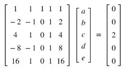
The solution vector 'X' is:

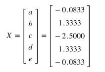
The value of `a=e` and `b=d`, also these values must be divided by `Deltax^2` to get right results. Substituting the values in our form gives

`(deltaf^2(x))/(deltax^2)=(-0.0833*f_(i-2)+1.3333*f_(i-1)-2.5*f_i+1.3333*f_(i+1)-0.0833*f_(i+2))/(Deltax^2)`.

To check the order of approximation, we must know the leading term ignored. To do so, lets write the taylor series approximation of `f(x)` and substitute the values of a,b,c,d. and e:

`(delta^2f(x))/(deltax^2)=(4*a+b+d+4*e)f''(x)(Deltax^2)/2+(-32*a-b+d+32*e)f^5(x)(Deltax^5)/(5!)+(64*a+b+d+64*e)f^6(x)(Deltax^6)/(6!) + ...`.

Coefficient of `f''(x)` is 1 and `a=e` and `b=d` which makes coefficient of `f^5(x)` to be 0. The coefficient of `f^6(x)` is non-zero (-7.9958/6!). Thus,

`a*f_(i-2)+b*f_(i-1)+c*f_i+d*f_(i+1)+e*f_(i+2) =` `(4*a+b+d+4*e)f''(x)(Deltax^2)/2+(64*a+b+d+64*e)f^6(x)(Deltax^6)/(6!) + ...`

Dividing by `Deltax^2` we get ,

`(a*f_(i-2)+b*f_(i-1)+c*f_i+d*f_(i+1)+e*f_(i+2))/(Deltax^2) = (4*a+b+d+4*e)(f''(x))/2+(64*a+b+d+64*e)f^6(x)(Deltax^4)/(6!) + ...`

After rearranging the terms we get,

`(deltaf^2(x))/(deltax^2)=(a*f_(i-2)+b*f_(i-1)+c*f_i+d*f_(i+1)+e*f_(i+2))/(Deltax^2) + O(Deltax^4)`.

Therefore, our scheme is of fourth-order as leading term ignored contains `Deltax^4`.

2. Skewed right hand difference : To compute fourth-order approximation of skewed right hand difference, we need 5 points ahead of current location. Thus stencil of 6 points will be used. Let `Deltax` be spacing. The general form of approximation is:

`(d^2f(x))/(dx^2) approx (delta^2f(x))/(deltax^2)=a*f_(i)+b*f_(i+1)+c*f_(i+2)+d*f_(i+3)+e*f_(i+4)+h*f_(i+5)`. To compute the values of a,b,c,d,e,h, we use Taylor table:

`(delta^2f(x))/(deltax^2)`	`f(x)`	`f^'(x)Deltax`	`f^('')(x)(Deltax^2)/(2!)`	`f^(''')(x)(Deltax^3)/(3!)`	`f^(4)(x)(Deltax^4)/(4!)`	`f^(5)(x)(Deltax^5)/(5!)`	`f^(6)(x)(Deltax^6)/(6!)`	`f^(7)(x)(Deltax^7)/(7!)`
`a*f_(i)`	`a`	`0`	`0`	`0`	`0`	`0`	`0`	`0`
`b*f_(i+1)`	`b`	`b`	`b`	`b`	`b`	`b`	`b`	`b`
`c*f_(i+2)`	`c`	`2*c`	`4*c`	`8*c`	`16*c`	`32*c`	`64*c`	`128*c`
`d*f_(i+3)`	`d`	`3*d`	`9*d`	`27*d`	`81*d`	`243*d`	`729*d`	`2187*d`
`e*f_(i+4)`	`e`	`4*e`	`16*e`	`64*e`	`256*e`	`1024*e`	`4096*e`	`16384*e`
`h*f_(i+5)`	`h`	`5*h`	`25*h`	`125*h`	`625*h`	`3125*h`	`15625*h`	`78125*h`
`sum`	`0`	`0`	`1`	`0`	`0`	`0`	`?`	`?`

Since, there are 6 unknowns to solve, we ignore derivatives higher than five as they are sufficient to solve the equations. The equations are:

`a+b+c+d+e+h=0 -> (1)`

`b+2*c+3*d+4*e+5*h=0 ->(2)`

`(b+4*c+9*d+16*e+25*h)*Deltax^2=2->(3)`

`b+8*c+27*d+64*e+125*h=0->(4)`

`b+16*c+81*d+256*e+625*h=0->(5)`

`b+32*c+243*d+1024*e+3125*h=0->(6)`.

For convenience, we ignore `Deltax^2` term in Eqn.(3) as other eqn's can also be multiplied by `Deltax^2` without loss or change in solution and we will later divide the solution by `Deltax^2`.

Solving system of above equations in matrix form results: AX = B ;

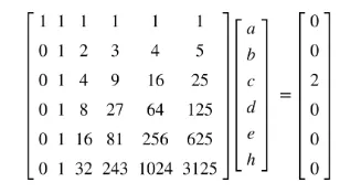
The solution vector 'X' is:

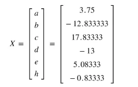
These values must be divided by `Deltax^2`. Substituting these values in our general form, we get:

`(d^2f(x))/(dx^2) approx (delta^2f(x))/(deltax^2)=(3.75*f_(i)-12.833333*f_(i+1)+17.83333*f_(i+2)-13*f_(i+3)+5.08333*f_(i+4)-0.83333*f_(i+5))/(Deltax^2)`

To check the order of approximation, we must know the leading term ignored. To do so, lets write the taylor series approximation of `f(x)` and substitute the values of a,b,c,d,e and h:

`(delta^2f(x))/(deltax^2)=(b+4*c+9*d+16*e+25*h)f''(x)(Deltax^2)/2+(b+64*c+729*d+4096*e+15625*h)f^6(x)(Deltax^6)/(6!)``+(b+128*c+2187*d+16384*e+78125*h)f^7(x)(Deltax^7)/(7!) + ...`

The coefficient of `f''(x)` is 1 and the coefficient of `f^6(x)` is non-zero (-547.96/6!). Thus,

`a*f_(i)+b*f_(i+1)+c*f_(i+2)+d*f_(i+3)+e*f_(i+4)+h*f_(i+5)` = `(b+4*c+9*d+16*e+25*h)f''(x)(Deltax^2)/2+(b+64*c+729*d+4096*e+15625*h)f^6(x)(Deltax^6)/(6!)+...`.

Dividing by `Deltax^2` we get,

`(a*f_(i)+b*f_(i+1)+c*f_(i+2)+d*f_(i+3)+e*f_(i+4)+h*f_(i+5))/(Deltax^2)` = `(b+4*c+9*d+16*e+25*h)(f''(x))/2+(b+64*c+729*d+4096*e+15625*h)f^6(x)(Deltax^4)/(6!)+...`.

After rearranging these terms we get:

`(deltaf^2(x))/(deltax^2)=(a*f_(i)+b*f_(i+1)+c*f_(i+2)+d*f_(i+3)+e*f_(i+4)+h*f_(i+5))/(Deltax^2) + O(Deltax^4)`.

Therefore, our scheme is of fourth-order as leading term ignored contains `Deltax^4`.

3. Skewed Left side difference : To compute fourth-order approximation of skewed left hand difference, we need 5 points behind of current location. Thus stencil of 6 points will be used. Let `Deltax` be spacing. The general form of approximation is:

`(d^2f(x))/(dx^2) approx (delta^2f(x))/(deltax^2)=a*f_(i-5)+b*f_(i-4)+c*f_(i-3)+d*f_(i-2)+e*f_(i-1)+h*f_(i)`. To compute the values of a,b,c,d,e,h, we use Taylor table:

`(delta^2f(x))/(deltax^2)`	`f(x)`	`f^'(x)Deltax`	`f^('')(x)(Deltax^2)/(2!)`	`f^(''')(x)(Deltax^3)/(3!)`	`f^(4)(x)(Deltax^4)/(4!)`	`f^(5)(x)(Deltax^5)/(5!)`	`f^(6)(x)(Deltax^6)/(6!)`	`f^(7)(x)(Deltax^7)/(7!)`
`a*f_(i-5)`	`a`	`-5*a`	`25*a`	`-125*a`	`625*a`	`-3125*a`	`15625*a`	`-78125*a`
`b*f_(i-4)`	`b`	`-4*b`	`16*b`	`-64*b`	`256*b`	`-1024*b`	`4096*b`	`-16384*b`
`c*f_(i-3)`	`c`	`-3*c`	`9*c`	`-27*c`	`81*c`	`-243*c`	`729*c`	`-2187*c`
`d*f_(i-2)`	`d`	`-2*d`	`4*d`	`-8*d`	`16*d`	`-32*d`	`64*d`	`-128*d`
`e*f_(i-1)`	`e`	`-e`	`e`	`-e`	`e`	`-e`	`e`	`-e`
`h*f_(i)`	`h`	`0`	`0`	`0`	`0`	`0`	`0`	`0`
`sum`	`0`	`0`	`1`	`0`	`0`	`0`	`?`	`?`

Since, there are 6 unknowns to solve, we ignore derivatives higher than five as they are sufficient to solve the equations. The equations are:

`a+b+c+d+e+h=0 -> (1)`

`-5*a-4*b-3*c-2*d-e=0 ->(2)`

`(25*a+16*b+9*c+4*d+e)*Deltax^2=2->(3)`

`-125*a-64*b-27*c-8*d-e=0->(4)`

`625*a+256*b+81*c+16*D+e=0->(5)`

`-3125*a-1024*b-243*c-32*d-e=0->(6)`.

For convenience, we ignore `Deltax^2` term in Eqn.(3) as other eqn's can also be multiplied by `Deltax^2` without loss or change in solution and we will later divide the solution by `Deltax^2`.

Solving system of above equations in matrix form results: AX = B ;

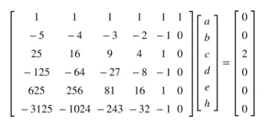
The solution vector 'X' is:

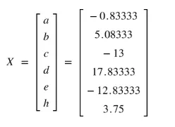
These values must be divided by `Deltax^2`. Substituting these values in our general form, we get:

`(d^2f(x))/(dx^2) approx (delta^2f(x))/(deltax^2)=(-0.83333*f_(i-5)+5.08333*f_(i-4)-13*f_(i-3)+17.83333*f_(i-2)-12.83333*f_(i-1)+3.75*f_(i))/(Deltax^2)`

To check the order of approximation, we must know the leading term ignored. To do so, let's write the Taylor series approximation of `f(x)` and substitute the values of a,b,c,d,e, and h:

`(delta^2f(x))/(deltax^2)=(25*a+16*b+9*c+4*d+e)f''(x)(Deltax^2)/2+(15625*a+4096*b+729*c+64*d+e)f^6(x)(Deltax^6)/(6!)``+(-78125*a-16384*b-2187*c-128*d-e)f^7(x)(Deltax^7)/(7!) + ...`.

The coefficient of `f''(x)` is 1 and the coefficient of `f^6(x)` is non-zero (-547.96/6!). Thus,

`a*f_(i-5)+b*f_(i-4)+c*f_(i-3)+d*f_(i-2)+e*f_(i-1)+h*f_i=``(25*a+16*b=9*c+4*d+e)f''(x)(Deltax^2)/2+(15625*a+4096*b+729*c+64*d+e)f^6(x)(Deltax^6)/(6!)+...`

Dividing by `Deltax^2` we get,

`(a*f_(i-5)+b*f_(i-4)+c*f_(i-3)+d*f_(i-2)+e*f_(i-1)+h*f_i)/(Deltax^2)=` `(25*a+16*b=9*c+4*d+e)(f''(x))/2+(15625*a+4096*b+729*c+64*d+e)f^6(x)(Deltax^4)/(6!)+...`,

After rearranging these terms we get:

`(deltaf^2(x))/(deltax^2)=(a*f_(i-5)+b*f_(i-4)+c*f_(i-3)+d*f_(i-2)+e*f_(i-1)+h*f_i)/(Deltax^2) + O(Deltax^4)`.

Therefore, our scheme is of fourth-order as leading term ignored contains `Deltax^4`.

• Now, we can make use of hint to prove the order of approximation. For central difference, we used 5 stencil points. Therefore,order of accuracy = 5 - 2(derivative order) + 1 = 4.
• For skewed right and left-hand difference, no of stencil points are 6. Therefore, order of accuracy = 6 - 2(order of derivative) = 4.
• Thus, instead of deriving order of accuracy by some tedious methods, the above thumb rule can be used.
• The central difference requires 1 less stencil point to have the same order of accuracy compared to skewed difference. Also since left and right-skewed difference are a mirror images of each other and have a same number of stencil points, they have the same order of accuracy.

MATLAB CODE:

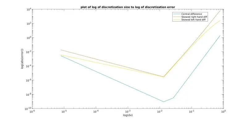
The main code "main_second_derivative.m" initializes the value of parameters x, dx and calls the function to calculate the respective approximation error. Then it plots the log of error vs the log of dx.

clc;
close all;
clear all;

% main code where x and dx are assigned and function to find second
% derivative taylor series approximation is called.

x = 2*pi;
dx = linspace(pi/4,pi/400000,60);        % range of dx

error = zeros(length(dx),3);            % [central right left]

% call to function
for j = 1:length(dx)
          error(j,1) = second_derivative_central_approx(x,dx(j));
          error(j,2) = second_derivative_right_approx(x,dx(j));
          error(j,3) = second_derivative_left_approx(x,dx(j));
end
    
loglog(dx,error(:,1),dx,error(:,2),dx,error(:,3));
xlabel('log(dx)');
ylabel('log(abs(error))');
title('plot of log of discretization size to log of discretization error');
legend('Central difference','Skewed right hand diff','Skewed left hand diff');

%%%%%%%%%%%%%%%%%%%%%%%%%%%%%%%%%%%%%%%%%%%%%%%%%%%%%%%%%%%%%%%%%%%%%%%%%%%%%%%%%%

The function's "second_derivative_central_approx" , "second_derivative_right_approx", "second_derivative_left_approx" first calculates the coefficient from taylor table using AX = B, then return the absolute value of error. The function also calculates the exact value of function.

1. Central difference :

% Function to calculate 4th order central difference

function err = second_derivative_central_approx(x,dx)

exact_value = -2*exp(x)*sin(x);    % f(x) = exp(x)*cos(x)

% Taylor table matrices
A = [1 1 1 1 1; -2 -1 0 1 2;4 1 0 1 4; -8 -1 0 1 8; 16 1 0 1 16];  % Taylor table matrix
B = [0; 0; 2; 0; 0];
X = A\B;                                                            % coefficient vector
  
% function values at nodes
f1 = exp(x-2*dx)*cos(x-2*dx);                   % f(x-2dx)
f2 = exp(x-dx)*cos(x-dx);                       % f(x-dx)
f3 = exp(x)*cos(x);                             % f(x)
f4 = exp(x+dx)*cos(x+dx);                       % f(x+dx)
f5 = exp(x+2*dx)*cos(x+2*dx);                   % f(x+2dx)

fourth_order_central_approx = (X(1)*f1 + X(2)*f2 + X(3)*f3 + X(4)*f4 + X(5)*f5)/dx^2;
err = abs(exact_value - fourth_order_central_approx);

end

2. Skewed right-hand difference :

% Function to calculate 4th order skewed right hand difference

function err = second_derivative_right_approx(x,dx)

exact_value = -2*exp(x)*sin(x);    % f(x) = exp(x)*cos(x)

% Taylor table matrices
A = [1 1 1 1 1 1; 0 1 2 3  4 5; 0 1 4 9 16 25; 0 1 8 27 64 125; 0 1 16 81 256 625; 0 1 32 243 1024 3125];  % Taylor table matrix
B = [0; 0; 2; 0; 0; 0];
X = A\B;                                                            % coefficient vector
  
% function values at nodes
f1 = exp(x)*cos(x);                             % f(x)
f2 = exp(x+dx)*cos(x+dx);                       % f(x+dx)
f3 = exp(x+2*dx)*cos(x+2*dx);                   % f(x+2dx)
f4 = exp(x+3*dx)*cos(x+3*dx);                   % f(x+3dx)
f5 = exp(x+4*dx)*cos(x+4*dx);                   % f(x+4dx)
f6 = exp(x+5*dx)*cos(x+5*dx);                   % f(x+5dx)

fourth_order_right_approx = (X(1)*f1 + X(2)*f2 + X(3)*f3 + X(4)*f4 + X(5)*f5 +X(6)*f6)/dx^2;
err = abs(exact_value - fourth_order_right_approx);

end

3. Skewed left-hand difference :

% Function to calculate 4th order skewed left hand difference

function err = second_derivative_left_approx(x,dx)

exact_value = -2*exp(x)*sin(x);    % f(x) = exp(x)*cos(x)

% Taylor table matrices
A = [1 1 1 1 1 1; -5 -4 -3 -2 -1 0; 25 16 9 4 1 0; -125 -64 -27 -8 -1 0; 625 256 81 16 1 0; -3125 -1024 -243 -32 -1 0];  % Taylor table matrix
B = [0; 0; 2; 0; 0; 0];
X = A\B;                                                            % coefficient vector

% function value at nodes
f1 = exp(x-5*dx)*cos(x-5*dx);                             % f(x-5dx)
f2 = exp(x-4*dx)*cos(x-4*dx);                             % f(x-4dx)
f3 = exp(x-3*dx)*cos(x-3*dx);                             % f(x-3dx)
f4 = exp(x-2*dx)*cos(x-2*dx);                             % f(x-2dx)
f5 = exp(x-dx)*cos(x-dx);                                 % f(x-dx)
f6 = exp(x)*cos(x);                                       % f(x)

fourth_order_left_approx = (X(1)*f1 + X(2)*f2 + X(3)*f3 + X(4)*f4 + X(5)*f5 +X(6)*f6)/dx^2;
err = abs(exact_value - fourth_order_left_approx);

end

OUTPUT :

EXPLANATION :

• Theoretically, all three methods are of fourth-order, so with a reduction in step size, the error reduces with the same factor for all (i.e factor of `1/n^4` where n is a factor in step size reduction). However, from the plot, it is quite visible that central difference gives even lower values of error than skewed right and left difference. One reason is might be the coefficient magnitude of the leading term since the numerical error is the sum of truncation error and round-off error and the coefficient magnitude of the leading term ignored contributes to truncation error and computers contributes to round-off error. For central difference, the coefficient magnitude of the leading term is 7.9968/6! and that of right, the left difference is 547.96/6!. The coefficient magnitude of the leading term is smaller for the central difference compared to the right and left difference. Therefore, the central difference has less truncation error and the total error is less than the skewed difference.
• After some value of discrete step size, further reduction leads to an increase in error in all their approximation method. For the central difference, the increase is much greater than the skewed difference. This is due to fact that error consists of two parts: truncation error and round-off error. As step size reduces to a very low value, the round-off error increases and forms a major contributor to the error term. For central difference, round off errors is greater than skewed difference.
• Skewed schemes are useful over central difference schemes where the nodes are not available on both sides of the point of concern. Such nodes exist on physical boundaries for spatial discretization.

Summary:

• Central difference scheme has a lower magnitude of truncation error than the skewed scheme. But at a very less step size, the central difference scheme contributes more round-off error than the skewed scheme.
• The central difference scheme cannot be used at the boundaries of the domain.