Week 7 - Simulation of a 1D Super-sonic nozzle flow simulation using Macormack Method

1-D quasi isentropic flow through convergent-divergent nozzle already has an analytical solution and is one of well studied physical phenomenon and system. Thus, if we could solve the governing equations that govern the quasi-isentropic flow through the C-D nozzle and compare the flow field obtained with analytical results, good confidence on numerical methods can be developed, and also a comparison study can be done between different forms of governing equations (non-conservation vs conservation form). Although these forms are theoretically the same, they behave differently in the numerical domain and hence require a comparative study.

Consider the C-D nozzle as shown in the figure below :

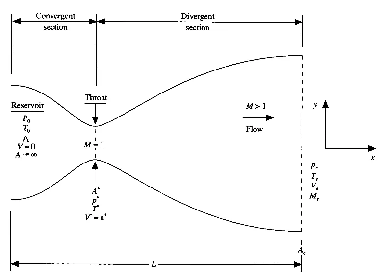
As shown, there is inlet condition as a reservoir, the convergent section has a subsonic condition, at throat Mach number is 1 (sonic), the divergent section has supersonic flow condition.

To derive governing equations, consider the control volume shown in the figure below;

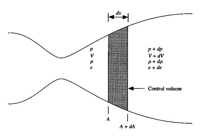
1. CONSERVATION FORM:

• Continuity equation:`(del(rho^'A^'))/(delt^')+(del(rho^'A^'V^'))/(delx^') = 0`.
• Momentum equation:`(del(rho^'A^'V^'))/(delt^')+(del(rho^'A^'V^('2) +1/gammap^'A^'))/(delx^') = 1/gammap^'(delA^')/(delx^')`.
• Energy equation:`(del(rho^'(e^'/(gamma-1)+(gammaV^('2))/2)A^'))/(delt^') + (del(rho^'(e^'/(gamma-1)+(gammaV^('2))/2)A^'V^' + p^'A^'V^'))/(delx^') = 0`.

2. NON-CONSERVATION FORM:

• Continuity equation: `(delrho^')/(delt^') +rho^'(delV^')/(delx^') + rho^'V^'(dellnA^')/(delx^')+V^'(delrho^')/(delx^') = 0`.
• Momentum equation: `(delV^')/(delt^')+ V^'(delV^')/(delx^') + 1/gamma((delT^')/(delx^') + T^'/(rho^')(delrho^')/(delx^') ) = 0`.
• Energy equation: `(delT^')/(delt^') + V^'(delT^')/(delx^') +(gamma-1)T^'((delV^')/(delx^') + V^'(del(lnA^'))/(delx^') ) = 0`.

These form are in non-dimensional forms. The variables are non-dimensionalised as follows:

• Energy (Temperature) : `e^' = T^' = T/T_0`.
• Density = `rho^' = rho/rho_0`.
• Velocity = `V^' = V/a_0`, where `a_0` is local speed of sound.
• Length = `x^' = x/L`.
• Time = `t^' = t/(L/a_0)`.
• Area = `A^' = A/A^star`.

The conservation form of governing equation does not have derivative's on primitive variables (`rho`,`V`,`T`) directly instead has derivatives on a combination of these primitive variables and their fluxes. (`rho^'A^'V^'`,etc). The solution to primitive variables is then derived from these solution vectors of conservation form. This makes conservation form take more computational time and complexity than non-conservation form. However, since the conservation form does not solve for primitive variables, it is the preferred form if some discontinuity is present in primitive variables.

The MacCorMack's method :

Consider the equation `(delf)/(delt) = (delf)/(delx)` to be solved numerically. `f(x,0)` be the initial profile. The MacCormack's method involve's following steps

• The predictor step : `((delf)/(delt))_(i,p) = (f_(i+1)- f_i)/(Deltax)`. Here the forward difference is used for spatial derivative's.
• The updated solution : `f_i^' = f_(i,old) + ((delf)/(delt))_(i,p)*Deltat`.
• The corrector step : `((delf)/(delt))_(i,c) = (f_(i)^'- f_(i-1)^')/(Deltax)`. Here backward difference is used for spatial derivative.
• The average step : `((delf)/(delt))_(i,avg) =0.5(((delf)/(delt))_(i,p) +((delf)/(delt))_(i,c))`.
• The solution step : `f_i = f_(i,old) + ((delf)/(delt))_(i,avg)*Deltat`.

Apply the required boundary conditions.

Using the MacCormack method to solve the conservation and non-conservation form. Since it is explicit in nature, the CFL condition governs the stability and puts an upper limit on the time step for a given grid size.

`CFL = (c+v)*(Deltat)/(Deltax) <=1`, where `c` is local speed of sound. The time step taken is the minimum of time steps calculated for each grid size using the flow velocity and sound velocity of that grid.

The CODE :

• The function 'non_conservation.m' takes length, no of grids, no of time steps, gamma, and CFL limit as input and outputs the steady-state solution of primitive variables, time variation of primitive variable values at throat and outlet. The function initializes the initial conditions required for density, velocity, temperature. It also creates an area profile. It uses the MacCormack method to solve the non-conservation form numerically. During each time iteration, it calculates the value of the time step using the CFL condition. It also plots the spatial variation of the mass rate at different time steps.
• The initial conditions used are :

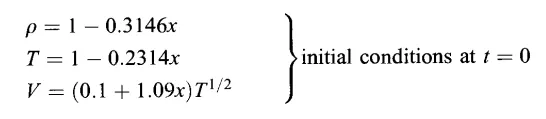
• The area profile is `A = 1 + 2.2(x - 1.5)^2` for `0<=x <=3`.
• Note: All calculations are done in non-dimensional form.

function [rho,v,T,P,mass_rate,M,throat_nc,outlet_nc] = non_conservation(L,n,nt,gamma,cfl)

x = linspace(0,L,n);
dx = x(2)-x(1);

% initial conditions
rho = 1 - 0.3146*x;
T = 1 - 0.2314*x;
v = (0.1+1.09*x).*T.^0.5;
P = rho.*T;
A = 1 + 2.2*(x - 1.5).^2;
mass_rate = rho.*A.*v;
c = T.^0.5;
M = v./c;

% Preallocation memories
drho_dt_p = zeros(1,n);
dv_dt_p = zeros(1,n);
dT_dt_p = zeros(1,n);
drho_dt_c = zeros(1,n);
dv_dt_c = zeros(1,n);
dT_dt_c = zeros(1,n);
throat_nc = zeros(6,nt);
outlet_nc = zeros(6,nt);

% figure(1)
for i = 1:nt
    
    % Recalculate value of time step;
    dt = min(cfl*dx./(c+v));
    
    % Keep track of old values of primitive parameters
    rho_old = rho;
    T_old = T;
    v_old = v;
    
    % Predictor step
    for j = 2:(n-1)
       drho_dx = (rho(j+1) - rho(j))/dx;
       dv_dx = (v(j+1) - v(j))/dx;
       dT_dx = (T(j+1) - T(j))/dx;
       dA_dx = (log(A(j+1)) - log(A(j)))/dx;
    
       drho_dt_p(j) = -rho(j)*dv_dx - rho(j)*v(j)*dA_dx - v(j)*drho_dx;
       dv_dt_p(j) = -v(j)*dv_dx - (dT_dx + T(j)*drho_dx/rho(j))/gamma;
       dT_dt_p(j) = -v(j)*dT_dx - (gamma - 1)*T(j)*(dv_dx + v(j)*dA_dx);
    
    % Updated solution
       rho(j) = rho_old(j) + drho_dt_p(j)*dt;
       v(j) = v_old(j) + dv_dt_p(j)*dt;
       T(j) = T_old(j) + dT_dt_p(j)*dt;
    end
    
    % Corrector step
    for j = 2:(n-1)
       drho_dx = (rho(j) - rho(j-1))/dx;
       dv_dx = (v(j) - v(j-1))/dx;
       dT_dx = (T(j) - T(j-1))/dx;
       dA_dx = (log(A(j)) - log(A(j-1)))/dx;
    
       drho_dt_c(j) = -rho(j)*dv_dx - rho(j)*v(j)*dA_dx - v(j)*drho_dx;
       dv_dt_c(j) = -v(j)*dv_dx - (dT_dx + T(j)*drho_dx/rho(j))/gamma;
       dT_dt_c(j) = -v(j)*dT_dx - (gamma - 1)*T(j)*(dv_dx + v(j)*dA_dx);
    end
    
    % Average values
    drho_dt = 0.5*(drho_dt_p + drho_dt_c);
    dv_dt = 0.5*(dv_dt_p + dv_dt_c);
    dT_dt = 0.5*(dT_dt_p + dT_dt_c);
    
    for j = 2:(n-1)
       rho(j) = rho_old(j) + drho_dt(j)*dt;
       v(j) = v_old(j) + dv_dt(j)*dt;
       T(j) = T_old(j) + dT_dt(j)*dt;
    end
    
    % Boundary Conditions
    % Inlet bc
    rho(1) = 1;
    T(1) = 1;
    v(1) = 2*v(2) - v(3);
    
    % Oulet bc
    rho(n) = 2*rho(n-1) - rho(n-2);
    v(n) = 2*v(n-1) - v(n-2);
    T(n) = 2*T(n-1) - T(n-2);
    
    % Update values of dependent variables
    P = rho.*T;
    c = T.^0.5;
    M = v./c;
    mass_rate = rho.*A.*v;
    
    % Time wise variation of properties at throat and outlet
    throat_nc(1,i) = rho(int16(n/2));
    throat_nc(2,i) = v(int16(n/2));
    throat_nc(3,i) = T(int16(n/2));
    throat_nc(4,i) = P(int16(n/2));
    throat_nc(5,i) = M(int16(n/2));
    throat_nc(6,i) = mass_rate(int16(n/2));
    
    outlet_nc(1,i) = rho(n);
    outlet_nc(2,i) = v(n);
    outlet_nc(3,i) = T(n);
    outlet_nc(4,i) = P(n);
    outlet_nc(5,i) = M(n);
    outlet_nc(6,i) = mass_rate(n);
    
    % plot time wise variation of mass flow rate inside nozzle
    figure(1)
    if i == 100
       plot(x, mass_rate, 'm', 'linewidth', 1.25);
       hold on
    elseif i == 200
       plot(x, mass_rate, 'c', 'linewidth', 1.25);
       hold on
    elseif i == 400
       plot(x, mass_rate, 'g', 'linewidth', 1.25);
       hold on
    elseif i == 800
       plot(x, mass_rate, 'y', 'linewidth', 1.25);
       hold on
    elseif i == 1200
       plot(x, mass_rate, 'k', 'linewidth', 1.25);
       hold on
    elseif i == 1400
       plot(x, mass_rate, 'r', 'linewidth', 1.25);
       hold on
    end
 
end
    title('Mass flow rates at different Timesteps - NON CONSERVATIVE FORM')
    xlabel('Distance')
    ylabel('Mass flow rate')
    legend({'100^t^h Timestep','200^t^h Timestep','400^t^h Timestep','800^t^h Timestep','1200^t^h Timestep','1400^t^h Timestep'})
    grid on    
end

• The function 'conservation.m' takes length, no of grids, no of time steps, gamma, and CFL limit as input and outputs the steady-state solution of primitive variables, time variation of primitive variable values at throat and outlet. The function initializes the initial conditions required for density, velocity, temperature. It also creates an area profile. It uses the MacCormack method to solve the conservation form numerically. During each time iteration, it calculates the value of the time step using the CFL condition. It also plots the spatial variation of the mass flow rate at different time steps.
• Since the solution vector is not primitive variables, they need to be calculated at the end of each time step. Boundary conditions are provided on solution variables and not primitive variables, unlike the non-conservation form.
• The initial conditions used are :

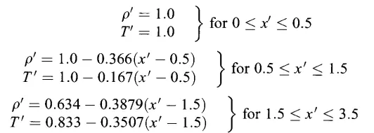
These conditions are used to derive initial conditions on the solution space of the conservation form.

• The initial condition on velocity is : `V^' = 0.59/(rho^'A^')`.
• The area profile is `A = 1 + 2.2(x - 1.5)^2` for `0<=x <=3`.
• Note: All calculations are done in non-dimensional form.

function [rho_c,v_c,T_c,P_c,mass_rate_c,M_c,throat_c,outlet_c] = conservation(L,n,nt,gamma,cfl)

x = linspace(0,L,n);
dx = x(2)-x(1);

% Memory allocation
rho_c = zeros(1,n);
T_c = zeros(1,n);
dU1_dt_p = zeros(1,n);
dU2_dt_p = zeros(1,n);
dU3_dt_p = zeros(1,n);
dU1_dt_c = zeros(1,n);
dU2_dt_c = zeros(1,n);
dU3_dt_c = zeros(1,n);
throat_c = zeros(6,nt);
outlet_c = zeros(6,nt);

% initial conditions
for i = 1:n
    if x(i) <= 0.5
        rho_c(i) = 1;
        T_c(i) = 1;
    elseif x(i)> 0.5 && x(i) <= 1.5
        rho_c(i) = 1 - 0.366*(x(i)-0.5);
        T_c(i) = 1 - 0.167*(x(i)-0.5);
    elseif x(i) > 1.5
        rho_c(i) = 0.634 - 0.3879*(x(i) - 1.5);
        T_c(i) = 0.833 - 0.3507*(x(i) - 1.5);
    end
end       
P_c = rho_c.*T_c;
A = 1 + 2.2*(x - 1.5).^2;
v_c = 0.59./(rho_c.*A);
mass_rate_c = rho_c.*A.*v_c;
speed = (T_c).^0.5;
M_c= v_c./speed;

% Initial solution vectors
U1 = rho_c.*A;
U2 = mass_rate_c;
U3 = rho_c.*(T_c/(gamma-1) + gamma*v_c.*v_c/2).*A;

for i = 1:nt
    
    % Recalculate value of time step;
    dt = min(cfl*dx./(speed+v_c));
    
    % Keep track of old values of solution vectors
    U1_old = U1;
    U2_old = U2;
    U3_old = U3;
    
    % Calculationg flux vectors
    F1 = U2;
    F2 = U2.*U2./U1 + (gamma-1)*(U3 - gamma*U2.*U2./(U1*2))/gamma;
    F3 = gamma*U2.*U3./U1 - gamma*(gamma-1)*(U2.*U2.*U2)./(2*U1.*U1);
    
    % Predictor step
    for j = 2:(n-1)
       J2 = rho_c(j)*T_c(j)*(A(j+1) - A(j))/(dx*gamma);
       dU1_dt_p(j) = -(F1(j+1) - F1(j))/dx;
       dU2_dt_p(j) = -(F2(j+1) - F2(j))/dx + J2;
       dU3_dt_p(j) = -(F3(j+1) - F3(j))/dx;
    
    % Updated solution
       U1(j) = U1_old(j) + dU1_dt_p(j)*dt;
       U2(j) = U2_old(j) + dU2_dt_p(j)*dt;
       U3(j) = U3_old(j) + dU3_dt_p(j)*dt;
    end
    
    % ReCalculationg flux vectors ans primitive variables
    F1 = U2;
    F2 = U2.*U2./U1 + (gamma-1)*(U3 - gamma*U2.*U2./(U1*2))/gamma;
    F3 = gamma*U2.*U3./U1 - gamma*(gamma-1)*(U2.*U2.*U2)./(2*U1.*U1);
    rho_c = U1./A;
    v_c = U2./U1;
    T_c = (gamma-1)*(U3./U1 - gamma*v_c.*v_c/2);
    
    % Corrector step
    for j = 2:(n-1)
       J2 = rho_c(j)*T_c(j)*(A(j) - A(j-1))/(dx*gamma);
       dU1_dt_c(j) = -(F1(j) - F1(j-1))/dx;
       dU2_dt_c(j) = -(F2(j) - F2(j-1))/dx + J2;
       dU3_dt_c(j) = -(F3(j) - F3(j-1))/dx;
    end
    
    % Average values
    dU1_dt = 0.5*(dU1_dt_p + dU1_dt_c);
    dU2_dt = 0.5*(dU2_dt_p + dU2_dt_c);
    dU3_dt = 0.5*(dU3_dt_p + dU3_dt_c);
    
    for j = 2:(n-1)
       U1(j) = U1_old(j) + dU1_dt(j)*dt;
       U2(j) = U2_old(j) + dU2_dt(j)*dt;
       U3(j) = U3_old(j) + dU3_dt(j)*dt;
    end
    
    % Boundary Conditions
    % Inlet bc
    U1(1) = A(1);
    U2(1) = 2*U2(2) - U2(3);
    U3(1) = U1(1)*(T_c(1)/(gamma-1) + gamma*(U2(1)*U2(1))/(2*U1(1)*U1(1)));
    
    % Oulet bc
    U1(n) = 2*U1(n-1) - U1(n-2);
    U2(n) = 2*U2(n-1) - U2(n-2);
    U3(n) = 2*U3(n-1) - U3(n-2);
    
    % Calculate values of primitive variables
    rho_c = U1./A;
    v_c = U2./U1;
    T_c = (gamma-1)*(U3./U1 - gamma*v_c.*v_c/2);
    P_c = rho_c.*T_c;
    speed = (T_c).^0.5;
    M_c = v_c./speed;
    mass_rate_c = U2;
    
    % Time wise variation of properties at throat and outlet
    [Value,throat_index] = min(A);
    throat_c(1,i) = rho_c(throat_index);
    throat_c(2,i) = v_c(throat_index);
    throat_c(3,i) = T_c(throat_index);
    throat_c(4,i) = P_c(throat_index);
    throat_c(5,i) = M_c(throat_index);
    throat_c(6,i) = mass_rate_c(throat_index);
    
    outlet_c(1,i) = rho_c(n);
    outlet_c(2,i) = v_c(n);
    outlet_c(3,i) = T_c(n);
    outlet_c(4,i) = P_c(n);
    outlet_c(5,i) = M_c(n);
    outlet_c(6,i) = mass_rate_c(n);
    
    % plot time wise variation of mass flow rate inside nozzle
    figure(3)
    if i == 100
       plot(x, mass_rate_c, 'm', 'linewidth', 1.25);
       hold on
    elseif i == 200
       plot(x, mass_rate_c, 'c', 'linewidth', 1.25);
       hold on
    elseif i == 400
       plot(x, mass_rate_c, 'g', 'linewidth', 1.25);
       hold on
    elseif i == 800
       plot(x, mass_rate_c, 'y', 'linewidth', 1.25);
       hold on
    elseif i == 1200
       plot(x, mass_rate_c, 'k', 'linewidth', 1.25);
       hold on
    elseif i == 1400
       plot(x, mass_rate_c, 'r', 'linewidth', 1.25);
       hold on
    end
 
end
    title('Mass flow rates at different Timesteps - CONSERVATIVE FORM')
    xlabel('Distance')
    ylabel('Mass flow rate')
    legend({'100^t^h Timestep','200^t^h Timestep','400^t^h Timestep','800^t^h Timestep','1200^t^h Timestep','1400^t^h Timestep'})
    grid on    
end

• The main code 'main_nozzle.m' initialize the parameters like length of the domain, no of spatial steps, and time steps, cfl value. Calls the above two functions. The output from both the functions are the steady-state solution of density, velocity, temperature, pressure, Mach number, mass flow rate, and time variation of these quantities at throat and outlet locations. The plots are the comparison between the steady-state solution of non-conservation and conservation form, time variation of primitive variables between both forms, mass flow rate comparison between two forms.

clc;
close all;
clear all;

% Parameters initialization
L = 3;                             % Length of domain
n = 31;                            % no of nodes
x = linspace(0,L,n);               
nt = 1400;                         % time steps
t = 1:nt;
gamma = 1.4;                       % property of gas
cfl = 0.5;                         % CFL number

% Call to function to solve non-ceonservation form
tic
[rho_nc,v_nc,T_nc,P_nc,mass_rate_nc,M_nc,throat_nc,outlet_nc] = non_conservation(L,n,nt,gamma,cfl);
nc_form = toc;

% Call to function to solve conservation form
tic
[rho_c,v_c,T_c,P_c,mass_rate_c,M_c,throat_c,outlet_c] = conservation(L,n,nt,gamma,cfl);
c_form = toc;

% PLotting steady state primitive variables in NC and C form
figure(2)
subplot(5,1,1)
plot(x,rho_nc,'c',x,rho_c,'r');
ylabel('Density');
legend('Non-conservation', 'Conservation');
title('Steady state distribution of primitive variables - Non conservation vs Conservation form');

subplot(5,1,2)
plot(x,v_nc,'c',x,v_c,'r');
ylabel('Velocity');
legend('Non-conservation', 'Conservation');

subplot(5,1,3)
plot(x,T_nc,'c',x,T_c,'r');
ylabel('Temperature');
legend('Non-conservation', 'Conservation');

subplot(5,1,4)
plot(x,P_nc,'c',x,P_c,'r');
ylabel('Pressure');
legend('Non-conservation', 'Conservation');

subplot(5,1,5)
plot(x,M_nc,'c',x,M_c,'r');
ylabel('Mach number');
legend('Non-conservation', 'Conservation');

xlabel('distance');
grid on

% PLotting time variation primitive variables in NC form and C form at throat
figure(4)
subplot(5,1,1)
plot(t,throat_nc(1,:),'c',t,throat_c(1,:),'r');
ylabel('Density');
legend('Non-conservation', 'Conservation');
title('Time variation of primitive variables at throat - Non conservation vs Conservation form');

subplot(5,1,2)
plot(t,throat_nc(2,:),'c',t,throat_c(2,:),'r');
ylabel('Velocity');
legend('Non-conservation', 'Conservation');

subplot(5,1,3)
plot(t,throat_nc(3,:),'c',t,throat_c(3,:),'r');
ylabel('Temperature');
legend('Non-conservation', 'Conservation');

subplot(5,1,4)
plot(t,throat_nc(4,:),'c',t,throat_c(4,:),'r');
ylabel('Pressure');
legend('Non-conservation', 'Conservation');

subplot(5,1,5)
plot(t,throat_nc(5,:),'c',t,throat_c(5,:),'r');
ylabel('Mach number');
legend('Non-conservation', 'Conservation');

xlabel('time steps');
grid on

% Comparison plot of normalised mass flow rate for both form
figure(5)
subplot(2,1,1)
plot(x,mass_rate_nc,'c',x,mass_rate_c,'r');
xlabel('distance');
ylabel('Normalised mass flow rate');
legend('Non-consevation form','Conservation form');
title('Steady state mass flow rate comparison between non-conservation and conservation form');

subplot(2,1,2);
plot(t,throat_nc(6,:),'c',t,throat_c(6,:),'r');
xlabel('time steps');
ylabel('Normalised mass flow rate');
legend('Non-consevation form','Conservation form');
title('Time varying mass flow rate comparison between non-conservation and conservation form');

Plots :

• 1) For n (no of grids) = 31.

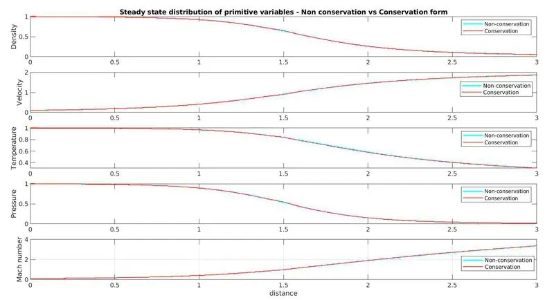
EXPLANATION: The steady-state values of primitive variables match in both forms. This concludes that both forms are numerically good to solve for steady-state solution till the CFL criterion is met.

Mach number is 1 at throat (x = 1.5). Before throat, flow is subsonic and after throat, flow is supersonic as seen in the Mach number plot. Also the pressure, density, temperature are reducing since the velocity is increasing. Hence this also shows that flow is quasi-isentropic throughout the C-D nozzle.

• 2) For n (no of grids) = 31. The values are at the throat.

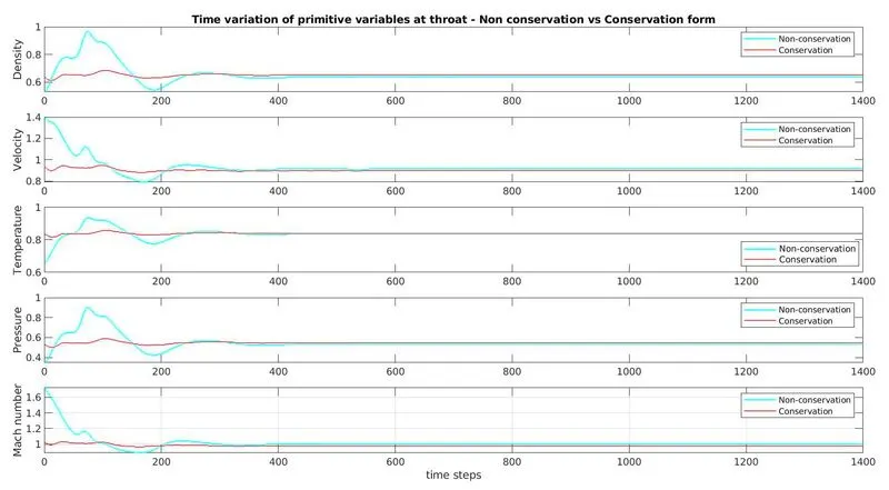
EXPLANATION: The non-conservation form shows oscillation (about steady-state) of much greater magnitude than the conservation form. Also, it takes more time for the non-conservation form to attain a steady-state than the conservation form. The steady-state value for both forms agrees with each other.

The conservation form is more stable than the non-conservation form.

• 3) Time variation of mass flow rate for both forms. n = 31.

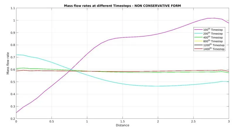
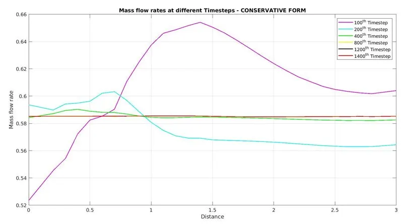
EXPLANATION: Both the forms take almost the same no of time iteration to converge to a steady-state value of mass flow rate (non-dimensional) (~ 0.586). However, consider the 100th iteration, the magnitude of deviation from steady-state solution for conservation form is much smaller than non-conservation form.

• 4) Normalised mass flow rate comparison. n = 31.

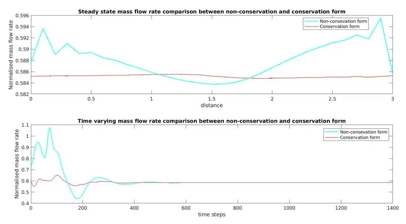
EXPLANATION: The first plot shows the comparison between mass flow rates for both same at steady-state along the length of the nozzle. The variation in steady-state solution for conservation form does not vary much along the length of the nozzle. But for the non-conservation form, this variation is much larger (~ +- 0.008).

The second plot is a time variation comparison in mass flow rate at the throat for both forms. At the start, the non-conservation form shows oscillation of a much larger magnitude than the conservation form and takes a greater no of iteration to converge to a steady-state value of close to 0.59. Conservation form is more stable than non-conservation form.

GRID DEPENDENCE TEST :

Grid Dependency test : Conditions at nozzle throat
Form	No of grids	Primitive variables (non-dimensional form)				Simulation time (sec)
		Density	Temperature	Pressure	Mach number
Non-conservation form	n = 31	0.6387	0.8365	0.5342	0.9994	1.752
	n = 61	0.6376	0.8354	0.5326	0.9997	1.684
Conservation form	n = 31	0.6504	0.8400	0.5463	0.9818	1.773
	n = 61	0.6383	0.8351	0.5330	0.9993	1.782
Expected value		0.634	0.833	0.528	1.000

A Grid-dependency test is done to ensure that the numerical method is independent of grid size. By reducing the grid size (increasing no of grid points), one tries to find at what level, the solution stops changing much even after further reduction in grid size. As shown in the above table, as no of grids is increased from 31 to 61, the solution goes closer to the expected value for both forms. Thus our method will result in a better solution at an even higher no of grid points and after which will become independent of no of the grid points. This is due to the reduction in truncation error as grid size is reduced.

For the conservation form, the simulation time is always higher than the non-conservation form. Thus, even though the conservation form is more stable than the non-conservation form, it takes a longer time.