Week 5.1 - Mid term project - Solving the steady and unsteady 2D heat conduction problem
- Steady-state heat conduction:
Consider a unit square domain. For steady heat conduction, the governing equation is:
`(del^2T)/(delx^2) + (del^2T)/(dely^2)=0`. Discretizing the elliptic pde (`b^2-4ac < 0`) with second order central difference, we get `(T_(i+1,j)-2*T_(i,j)+T_(i-1,j))/(Deltax^2)+(T_(i,j+1)-2*T_(i,j)+T_(i,j-1))/(Deltay^2) = 0`.
Denoting current node with letter `P` and for left, right, top, bottom nodes with `L`,`R`,`T`,`B` respectively, and arranging the terms we get, `T_P(2/(Deltax^2) + 2/(Deltay^2)) = (T_L+T_R)/(Deltax^2) + (T_T+T_B)/(Deltay^2)` -> (1).
To solve Eqn.(1), we use iterative solvers like Jacobi, gauss seidel, and SOR. Each iterative solver requires initial input. It stops when the solution between consecutive iterations does not change up to some magnitude decided by the user.
There is no stability problem in the discretized equation. However, the iterative solver might have its own pandora box. If the spectral radius of the iterative matrix for each iterative solver is less than 1, the solver is guaranteed to converge.
Algorithm for each iterative solver:
- Jacobi : `x_i^(k+1) = 1/a_(ii)(b_i-sum_(j!=i)a_(ij)x_j^k)`, where `k` is iteration step`
- Gauss Siedal = `x_i^(k+1) = 1/a_(ii)(b_i-sum_(j=1)^(i-1)a_(ij)x_j^(k+1)-sum_(j=i+1)^(n)a_(ij)x_j^k)`.
- SOR = `x_i^(k+1) = (1-omega)x_i^k + omega/a_(ii)(b_i-sum_(j=1)^(i-1)a_(ij)x_j^(k+1)-sum_(j=i+1)^(n)a_(ij)x_j^k)`.
CODE :
The function 'steady_solver.m' takes the initial guess of temperature field `T_(prev)`, iterative method, k1 (`1/(Deltax^2)`), k2 (`1/(Deltay^2)`), nodes in x and y direction (nx , ny) , tolerance to stop the iterative loop (tol) and omega as an over-relaxation factor. It implements the iterative method and after converging the solution returns the converged solution and no of iteration it took.
function [Tsol, iter] = steady_solver(Tprev,method,k1,k2,nx,ny,tol,omega)

term1 = 1/(2*k1+2*k2);
term2 = k1*term1;
term3 = k2*term1;
err = 10;
Told = Tprev;
T = Tprev;

if(method == 1)                          % jacobi
    jac_iter = 0;
    while err > tol
        for j = 2:(ny-1)
            for i = 2:(nx-1)
                H = Told(j,i-1) + Told(j,i+1);
                V = Told(j-1,i) + Told(j+1,i);
                T(j,i) = term2*H +term3*V;
            end
        end
        err = max(abs(T - Told),[],'all');
        Told = T;
        jac_iter = jac_iter + 1;
    end
    iter = jac_iter;

elseif(method == 2)                            % Gauss siedal
    gauss_iter = 0;
    while err > tol
        for j = 2:(ny-1)
            for i = 2:(nx-1)
                H = T(j,i-1) + Told(j,i+1);
                V = T(j-1,i) + Told(j+1,i);
                T(j,i) = term2*H +term3*V;
            end
        end
        err = max(abs(T - Told),[],'all');
        Told = T;
        gauss_iter = gauss_iter + 1;
    end
    iter = gauss_iter;

elseif(method == 3)                            % SOR
    sor_iter = 0;
    while err > tol
        for j = 2:(ny-1)
            for i = 2:(nx-1)
                H = T(j,i-1) + Told(j,i+1);
                V = T(j-1,i) + Told(j+1,i);
                T(j,i) = (1 - omega)*Told(j,i) + omega*(term2*H +term3*V);
            end
        end
        err = max(abs(T - Told),[],'all');
        Told = T;
        sor_iter = sor_iter + 1;
    end
    iter = sor_iter;
end

Tsol = T;
end
The main code 'steady_implicit.m' initializes the values of the parameters like length of the domain, the number of nodes in both directions, thermal diffusivity, grid size, tolerance, omega, boundary conditions, and initial temperature guess profile. Then it calls the above function with the required method. It also calculates the simulation time required. The plot is the temperature profile over the unit square domain.
%   2-D steady heat conduction problem over unit square
clear all;
close all;
clc;

% Parameters initialization
Lx  = 1;                                % x- length of domain
Ly = 1;                                 % y- length of domain
alpha = 1.1;                            % thermal diffusivity
nx = 100;                               % x-dir nodes
ny = 100;                               % y-dir nodes
x = linspace(0,Lx,nx);                  % x-coordinates
y = linspace(0,Ly,ny);                  % y-coordinates
dx = x(2)-x(1);                         % x-grid size
dy = y(2)-y(1);                         % y-grid size
k1 = 1/dx^2;
k2 = 1/dy^2;
tol = 10^-4;                            % tolerance for error check
omega = 1.9;                            % over relaxation parameter
% boundary conditions on domain
Tb = 900;                               % bottom face
Tl = 400;                               % left face
Tt = 600;                               % top face
Tr = 800;                               % right face

% Temperature varibale with boundary conditions
T = 300*ones(ny,nx);
T(1,:) = Tb;
T(:,1) = Tl;
T(end,:) = Tt;
T(:,end) = Tr;
% At corners, temperature is mean of adjacent faces
T(1,1) = (Tb + Tl)/2;
T(end,1) = (Tl + Tt)/2;
T(1,end) = (Tb + Tr)/2;
T(end,end) = (Tt + Tr)/2;

method = 3;                           % method 1 = jacobi, 2 = gauss siedal, 3 = sor

inner_iter = 0;
Tprev = T;
tic
% Call to function to iteratively solve temperature profile
[T, inner_iter] = steady_solver(Tprev, method, k1, k2, nx, ny, tol, omega);
simulation_time = toc;

% plot the contour of temperature
[M , c] = contourf(x,y,T);
clabel(M,c);
colorbar;
colormap(jet);
ax = gca;
xlabel('x-direction');
ylabel('y-direction');
if method == 3
    title_text = {'Steady heat conduction temperature profile';['Over-relaxation for sor: ',num2str(omega)];['No of iterations: ',num2str(inner_iter)]; ...
                 ['Simulation time: ', num2str(simulation_time),' s']};
else
    title_text = {'Steady heat conduction temperature profile';['Iteration method: ',num2str(method)];['No of iterations: ',num2str(inner_iter)]; ...
                 ['Simulation time: ', num2str(simulation_time),' s']};
end
title(title_text);
grid on;
Plots :
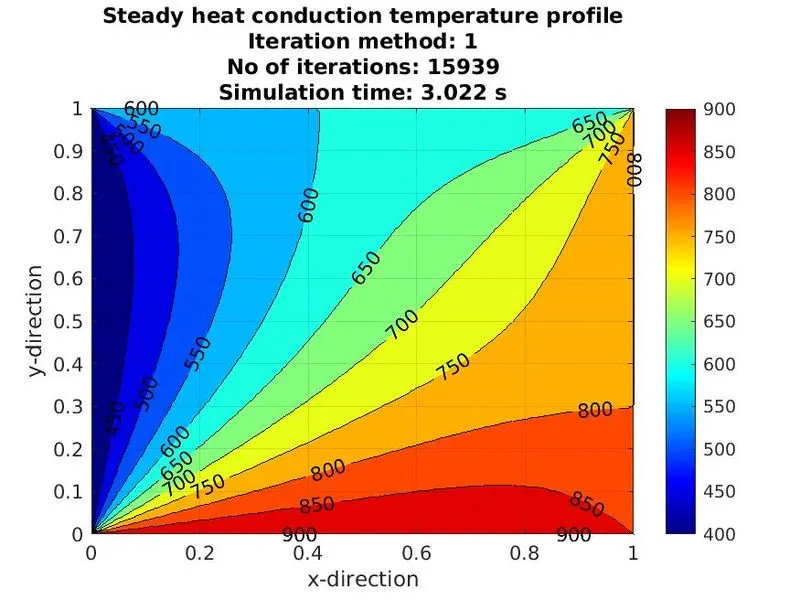
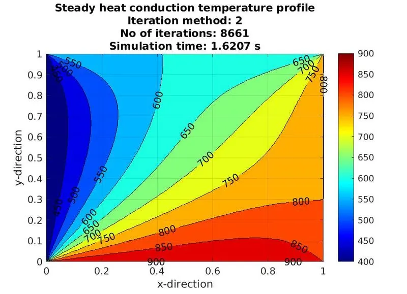
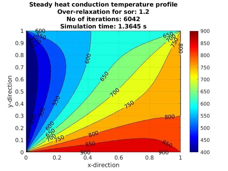
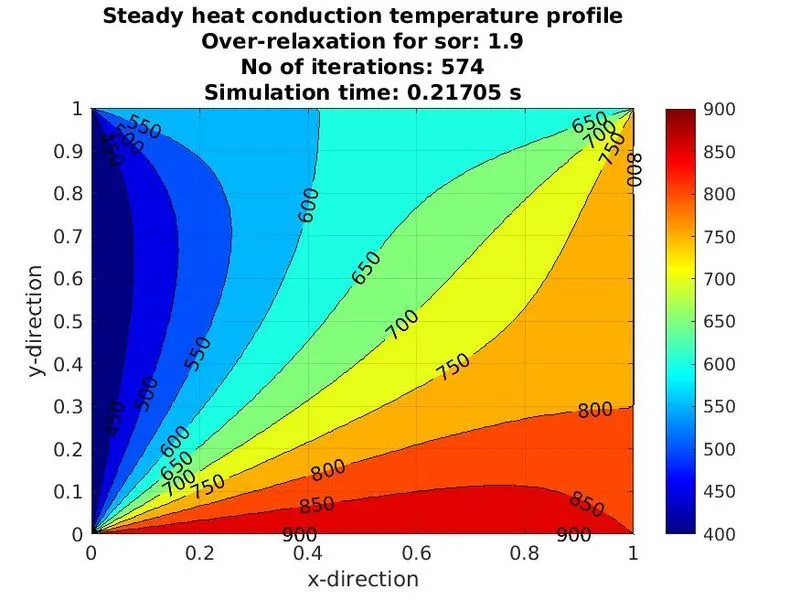
The above figure is a steady-state temperature profile. Important points to note are :
- In the figure with iteration method 1 (Jacobi), the iteration number is the largest among all. The second is gauss seidel and SOR has the least iterations for a converged solution as shown in the bottom figures.
- The same trend is shown by simulation time too as above.
- Even in SOR, with a change in over-relaxation factor omega, one can obtain a solution even faster. With omega 1.9, the solution converged faster than omega 1.2. So users might try a few omega and see how it affects the iteration number. With omega greater than 2, I was unable to get a converged solution.
- In the above figure, it can be seen that the inner domain is affected from all boundaries simultaneously, which is one of elliptic PDE nature.
- Transient Heat conduction (Explicit) :
The governing equation for transient heat conduction is `(delT)/(delt)=alpha((del^2T)/(delx^2) + (del^2T)/(dely^2))`, where `alpha` is thermal diffusivity. The pde requires time marching approach to solve numerically, with elliptic in nature spatial derivatives. So using forward difference in time and central difference for spatial coordinates with value at current time, we get `(T_(i,j)^(n+1)-T_(i,j)^n)/(Deltat)=alpha((T_(i+1,j)^n-2*T_(i,j)^n+T_(i-1,j)^n)/(Deltax^2)+(T_(i,j+1)^n-2*T_(i,j)^n+T_(i,j-1)^n)/(Deltay^2))`.
Denoting current node with letter `P` and for left, right, top, bottom nodes with `L`,`R`,`T`,`B` respectively, and arranging the terms we get, `T_P^(n+1)=(1-2k_1-2k_2)T_P^n+k1(T_R^(n)+T_L^n)+k2(T_T^(n)+T_B^n)` ->(2), where `k1 = (alphaDeltat)/(Deltax^2)` and `k2 = (alphaDeltat)/(Deltay^2)`.
To solve Eqn. (2), the initial condition is required. No iterative solver is needed. Since the discretization method is explicit in nature, stability concerns arise. The CFL condition is `k1+k2<=0.5`. So till the CFL condition is satisfied, the numerical method will result in a stable solution. Also, the CFL condition gives the relationship between time step and grid size. So for given grid size, the time step cannot be larger than required by CFL condition.
Code :
The code starts with parameter initialization like domain size (1*1), number of nodes (nx = 100, ny = 100) , thermal diffusivity (`alpha` = 1.1), grid size, k1, k2, time step (dt from k1 and k2 values), nt (time iterations), boundary conditions and initial temperature profile. The variable 'outer_iter' is used to loop over 'nt'. By deciding when to break from while loop using 'outer_iter' one can find both transient solution and steady-state solution. (e.g, if 'outer_iter <= nt' is used then the steady state is reached and if outer_iter <= nt/50'is used then transient solution is obtained). Physical time is calculated from 'outer_iter' and 'dt' values. The code also calculates simulation time. The total time (time to reach steady-state) is taken as 1 sec.
%   2-D unsteady heat conduction problem
clear all;
close all;
clc;

% Parameters initialization
Lx  = 1;                                % x- length of domain
Ly = 1;                                 % y- length of domain
alpha = 1.1;                            % thermal diffusivity
nx = 100;                               % x-dir nodes
ny = 100;                               % y-dir nodes
x = linspace(0,Lx,nx);                  % x-coordinates
y = linspace(0,Ly,ny);                  % y-coordinates
dx = x(2)-x(1);                         % x-grid size
dy = y(2)-y(1);                         % y-grid size
k1 = 0.2;                               % x-courant number
k2 = 0.2;                               % y-courant number
dt = (k1+k2)/(alpha/dx^2 + alpha/dy^2); % time step size
nt = 1/dt;                              % time iteration

% boundary conditions on domain
Tb = 900;                               % bottom face
Tl = 400;                               % left face
Tt = 600;                               % top face
Tr = 800;                               % right face

% Temperature varibale with boundary conditions
T = 300*ones(ny,nx);
T(1,:) = Tb;
T(:,1) = Tl;
T(end,:) = Tt;
T(:,end) = Tr;
% At corners, temperature is mean of adjacent faces
T(1,1) = (Tb + Tl)/2;
T(end,1) = (Tl + Tt)/2;
T(1,end) = (Tb + Tr)/2;
T(end,end) = (Tt + Tr)/2;

outer_iter = 0;

tic;
while outer_iter <= nt/50
    Told = T;
    for j = 2:(ny-1)
        for i = 2:(nx-1)
             H = Told(j,i-1) + Told(j,i+1);
             V = Told(j-1,i) + Told(j+1,i);
             T(j,i) = (1-2*k1-2*k2)*Told(j,i) + k1*H + k2*V;
         end
    end
    outer_iter = outer_iter  + 1;
end
simulation_time = toc;
% total time t
time = outer_iter*dt;

% plot the contour of temperature
[M , c] = contourf(x,y,T);
clabel(M,c);
colorbar;
colormap(jet);
ax = gca;
xlabel('x-direction');
ylabel('y-direction');
title_text = {'Transient heat conduction temperature profile';['Time: ', num2str(time),' s', '   time step :',num2str(dt),' s'];...
             ['CFL: ',num2str(k1+k2),'    Simulation time: ', num2str(simulation_time),' s']};
title(title_text);
grid on;
Plots :
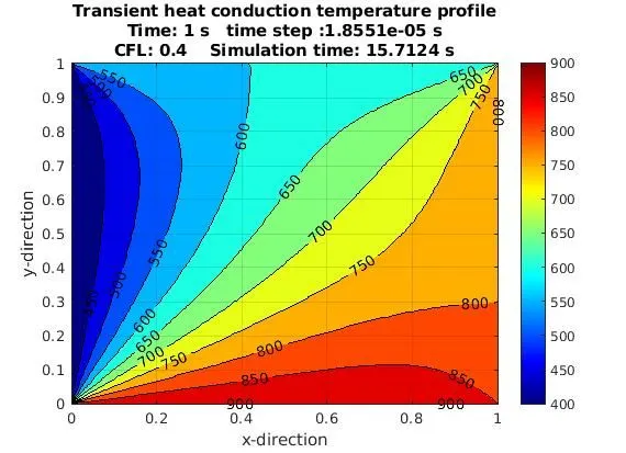
Figure (1)
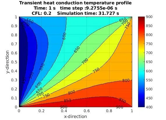
Figure (2)
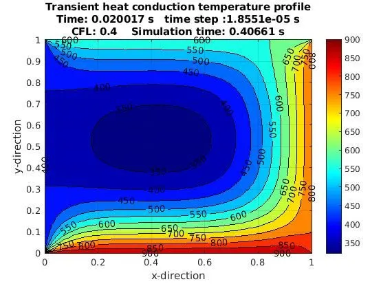
Figure (3)
- Figures (1) and (2) differs only in CFL conditions. Both are for end time 1 second where a steady-state solution exists. If the courant number is reduced by half, the time step reduces by half, and simulation time increases by 2 fold as expected.
- Figure (3) is for end time 0.02 seconds and courant number 0.4. It shows the transient solution. The Interior domain is close to 300 which is an initial condition used. Any other initial condition will give a transient solution of the interior domain close to that value. With time, due to diffusion, the solution reaches some steady-state solution.
- The Steady-state solution of the transient heat conduction problem in fig. (1) and (2) is very close to the solution obtained only by solving the steady-state heat conduction equation.
- Transient Heat conduction (Implicit) :
The governing equation for transient heat conduction is `(delT)/(delt)=alpha((del^2T)/(delx^2) + (del^2T)/(dely^2))`, where `alpha` is thermal diffusivity. The pde requires time marching approach to solve numerically, with elliptic in nature spatial derivatives. So using forward difference in time and central difference for spatial coordinates with value at current time, we get `(T_(i,j)^(n+1)-T_(i,j)^n)/(Deltat)=alpha((T_(i+1,j)^(n+1)-2*T_(i,j)^(n+1)+T_(i-1,j)^(n+1))/(Deltax^2)+(T_(i,j+1)^(n+1)-2*T_(i,j)^(n+1)+T_(i,j-1)^(n+1))/(Deltay^2))`.
Denoting current node with letter `P` and for left, right, top, bottom nodes with `L`,`R`,`T`,`B` respectively, and arranging the terms we get, `(1+2k_1+2k_2)T_P^(n+1)=T_P^n+k1(T_R^(n+1)+T_L^(n+1))+k2(T_T^(n+1)+T_B^(n+1))` ->(3), where `k1 = (alphaDeltat)/(Deltax^2)` and `k2 = (alphaDeltat)/(Deltay^2)`.
To solve Eqn.(3), we use iterative solvers like Jacobi, gauss seidel, and SOR. Each iterative solver requires initial input. It stops when the solution between consecutive iterations does not change up to some magnitude decided by the user.
The coefficient of the first term on the right-hand side in Eqn. (3) is always less than 1 irrespective value of `k_1, k_2`. So the method is unconditionally stable and no CFL condition is required to consider.
CODE :
The function 'Iterative_solver.m' takes the initial guess of temperature field `T_(prev)`, iterative method, k1 (`1/(Deltax^2)`), k2 (`1/(Deltay^2)`), nodes in x and y direction (nx , ny) , tolerance to stop the iterative loop (tol) and omega as an over-relaxation factor. It implements the iterative method and after converging the solution returns the converged solution and no of iteration it took.
function [Tsol, iter] = Iterative_solver(Tprev,method,k1,k2,nx,ny,tol,omega)

term1 = 1/(1+2*k1+2*k2);
term2 = k1*term1;
term3 = k2*term1;
err = 10;                                   % error
Told = Tprev;
T = Tprev;

if(method == 1)                              % jacobi
    jac_iter = 0;
    while err > tol
        for j = 2:(ny-1)
            for i = 2:(nx-1)
                H = Told(j,i-1) + Told(j,i+1);
                V = Told(j-1,i) + Told(j+1,i);
                T(j,i) = term1*Tprev(j,i) + term2*H +term3*V;
            end
        end
        err = max(abs(T - Told),[],'all');
        Told = T;
        jac_iter = jac_iter + 1;
    end
    iter = jac_iter;

elseif(method == 2)                            % Gauss siedal
    gauss_iter = 0;
    while err > tol
        for j = 2:(ny-1)
            for i = 2:(nx-1)
                H = T(j,i-1) + Told(j,i+1);
                V = T(j-1,i) + Told(j+1,i);
                T(j,i) = term1*Tprev(j,i) + term2*H +term3*V;
            end
        end
        err = max(abs(T - Told),[],'all');
        Told = T;
        gauss_iter = gauss_iter + 1;
    end
    iter = gauss_iter;

elseif(method == 3)                            % SOR
    sor_iter = 0;
    while err > tol
        for j = 2:(ny-1)
            for i = 2:(nx-1)
                H = T(j,i-1) + Told(j,i+1);
                V = T(j-1,i) + Told(j+1,i);
                T(j,i) = (1 - omega)*Told(j,i) + omega*(term1*Tprev(j,i) + term2*H +term3*V);
            end
        end
        err = max(abs(T - Told),[],'all');
        Told = T;
        sor_iter = sor_iter + 1;
    end
    iter = sor_iter;
end

Tsol = T;
end
The main code starts with parameter initialization like domain size (1*1), number of nodes (nx = 100, ny = 100) , thermal diffusivity (`alpha` = 1.1), grid size, k1, k2, time step (dt from k1 and k2 values), nt (time iterations), boundary conditions and initial temperature profile. The variable 'outer_iter' is used to loop over 'nt'. By deciding when to break from while loop using 'outer_iter' one can find both transient solution and steady-state solution. (e.g, if 'outer_iter <= nt' is used then steady state is reached and if outer_iter <= nt/50' is used then transient solution is obtained). Physical time is calculated from 'outer_iter' and 'dt' values. The code also calculates simulation time. The total time (time to reach steady-state) is taken as 1 sec. omega stores the over-relaxation factor for SOR.
%   2-D unsteady heat conduction problem on unit square
clear all;
close all;
clc;

% Parameters initialization
Lx  = 1;                                % x- length of domain
Ly = 1;                                 % y- length of domain
alpha = 1.1;                            % thermal diffusivity
nx = 100;                               % x-dir nodes
ny = 100;                               % y-dir nodes
x = linspace(0,Lx,nx);                  % x-coordinates
y = linspace(0,Ly,ny);                  % y-coordinates
dx = x(2)-x(1);                         % x-grid size
dy = y(2)-y(1);                         % y-grid size
k1 = 2;                               % x-courant number
k2 = 2;                               % y-courant number
dt = (k1+k2)/(alpha/dx^2 + alpha/dy^2); % time step size
nt = 1/dt;                              % time iteration
tol = 10^-4;                            % tolerance for error check
omega = 1.9;                            % over relaxation parameter
% boundary conditions on domain
Tb = 900;                               % bottom face
Tl = 400;                               % left face
Tt = 600;                               % top face
Tr = 800;                               % right face

% Temperature varibale with boundary conditions
T = 300*ones(ny,nx);
T(1,:) = Tb;
T(:,1) = Tl;
T(end,:) = Tt;
T(:,end) = Tr;
% At corners, temperature is mean of adjacent faces
T(1,1) = (Tb + Tl)/2;
T(end,1) = (Tl + Tt)/2;
T(1,end) = (Tb + Tr)/2;
T(end,end) = (Tt + Tr)/2;

method = 1;                           % method 1 = jacobi, 2 = gauss siedal, 3 = sor

outer_iter = 0;
inner_iter = 0;

tic;
while outer_iter <= nt/50
    Tprev = T;                        % previous step value initialization
    % call to function for iterative solution
    [T, iter] = Iterative_solver(Tprev, method, k1, k2, nx, ny, tol, omega);
    inner_iter = inner_iter + iter;
    outer_iter = outer_iter  + 1;
end
simulation_time = toc;
% total time t
time = outer_iter*dt;

% plot the contour of temperature
[M , c] = contourf(x,y,T);
clabel(M,c);
colorbar;
colormap(jet);
ax = gca;
xlabel('x-direction');
ylabel('y-direction');
if method == 3
    title_text = {'Transient heat conduction temperature profile';['Over-relaxation for sor: ',num2str(omega),'  Time :', num2str(time),' s'];...
                 ['Time step: ',num2str(dt),' s' ,'    No of iterations: ',num2str(inner_iter)]; ...
                 ['Simulation time: ', num2str(simulation_time),' s']};
else
    title_text = {'Transient heat conduction temperature profile';['Iteration method: ',num2str(method), '  Time :', num2str(time),' s'];...
                 ['Time step: ',num2str(dt),' s' ,'   No of iterations: ',num2str(inner_iter)]; ...
                 ['Simulation time: ', num2str(simulation_time),' s']};
end
title(title_text);
grid on;
PLOTS:
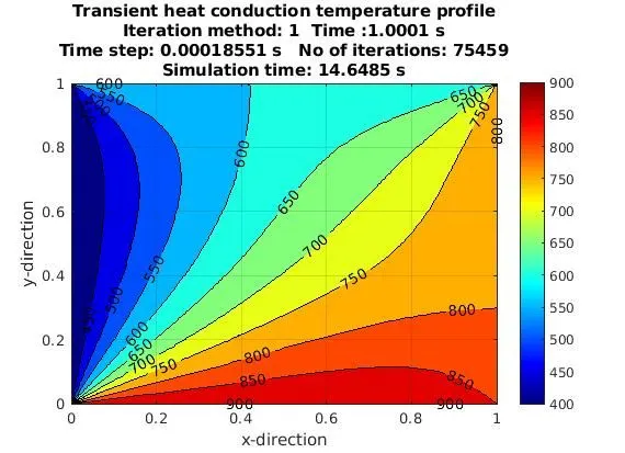
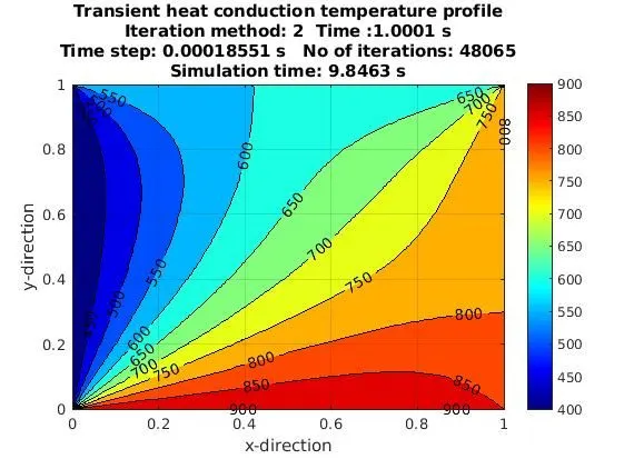
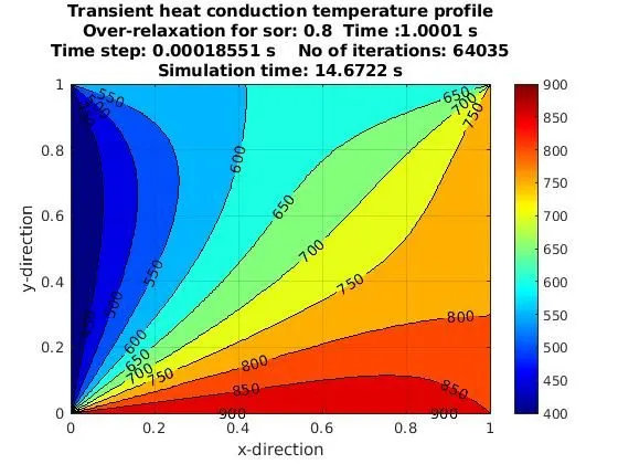
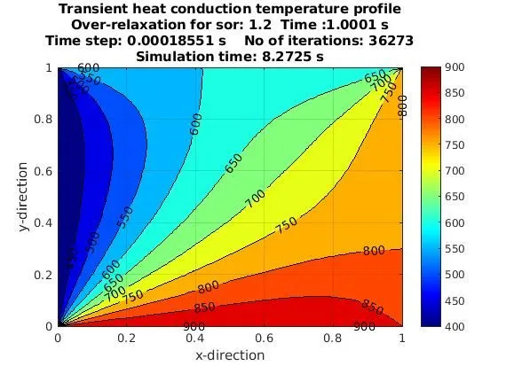
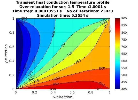
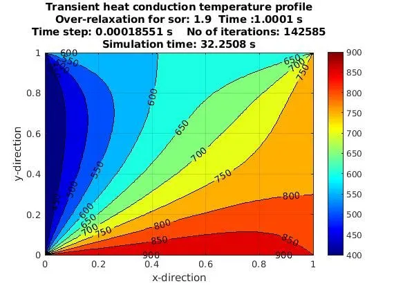
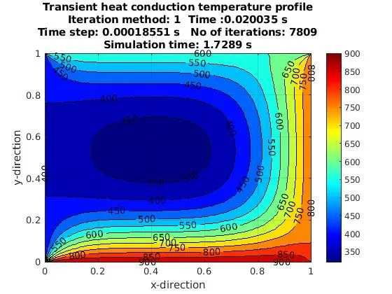
First six-figure show steady-state solutions for 3 iterative methods at an end time of 1 second.
- First, two figure's is for method 1 (Jacobi) and method 2 (gauss seidel). Gauss-Seidel takes less iteration and simulation time to give converged steady-state solution than Jacobi.
- The next four figures show the effect of the over-relaxation factor (omega) on no. of iterations and simulation time. For omega 0.8, SOR takes almost the same iterations and time as Jacobi. For omega 1.2, it takes lesser iterations and time than Gauss-Seidal. For omega 1.5, it takes even lesser iterations and simulation time than all before one, For omega 1.9, it takes more iterations and time than all. Thus, the omega value to be used should be close to 1.5 and on the lower side of it.
- The last figure shows the transient solution field at time 0.02 sec for method 1. The Interior domain is close to 300 which is an initial condition used. Any other initial condition will give the transient solution of the interior domain close to that value. With time, due to diffusion, the solution reaches some steady-state solution.
- The Steady-state solution of the transient heat conduction problem is very close to the solution obtained only by solving the steady-state heat conduction equation.