Week 8 - Simulating Cyclone separator with Discrete Phase Modelling
Aim :
1) To perform analysis on cyclone separator and calculate the separation efficiency and pressure drop.
2) To write a few words about any four empirical models used to calculate the cyclone separator efficiency.
3)To perform an analysis on a given cyclone separator model by varying the particle diameter from 1 μm to 5 μm and calculate the separation efficiency in each case and discuss the results.
4)To perform an analysis on a given cyclone separator model by varying the particle velocity from 1 m/sec to 5 m/sec and calculate the separation efficiency and pressure drop in each case and discuss the results.
Theory :
Cyclone separators or simply cyclones are separation devices that use the principle of inertia to remove particulate matter from flue gases. Cyclone separators is one of many air pollution control devices known as precleaners since they generally remove larger pieces of particulate matter. This prevents finer filtration methods from having to deal with large, more abrasive particles later on. In addition, several cyclone separators can operate in parallel, and this system is known as a multicyclone.
It is important to note that cyclones can vary drastically in their size. The size of the cyclone depends largely on how much flue gas must be filtered, thus larger operations tend to need larger cyclones. For example, several different models of one cyclone type can exist, and the sizes can range from a relatively small 1.2-1.5 m tall to around 9 meters .
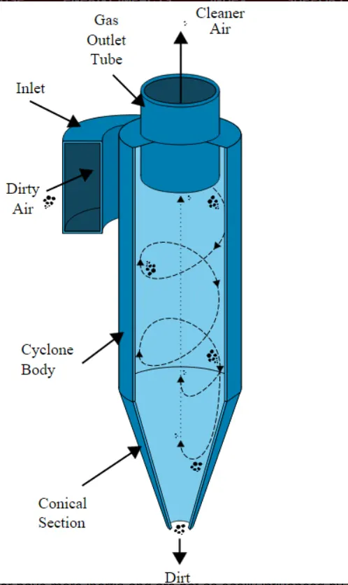
Cyclone separators work much like a centrifuge, but with a continuous feed of dirty air. In a cyclone separator, dirty flue gas is fed into a chamber. The inside of the chamber creates a spiral vortex, similar to a tornado. This spiral formation and the separation is shown in Figure 2. The lighter components of this gas have less inertia, so it is easier for them to be influenced by the vortex and travel up it. Contrarily, larger components of particulate matter have more inertia and are not as easily influenced by the vortex.
Since these larger particles have difficulty following the high-speed spiral motion of the gas and the vortex, the particles hit the inside walls of the container and drop down into a collection hopper. These chambers are shaped like an upside-down cone to promote the collection of these particles at the bottom of the container. The cleaned flue gas escapes out the top of the chamber.
Most cyclones are built to control and remove particulate matter that is larger than 10 micrometers in diameter. However, there do exist high efficiency cyclones that are designed to be effective on particles as small as 2.5 micrometers. As well, these separators are not effective on extremely large particulate matter. For particulates around 200 micrometers in size, gravity settling chambers or momentum separators are a better option.
Out of all of the particulate-control devices, cyclone separators are among the least expensive.They are often used as a pre-treatment before the flue gas enters more effective pollution control devices. Therefore, cyclone separators can be seen as "rough separators" before the flue gas reaches the fine filtration stages.
1) Emperical methods used to calculate cyclone seperator efficiency .
a) Iozia and Leith Model
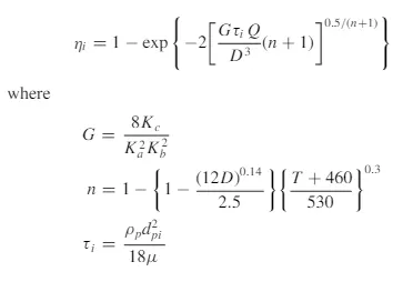
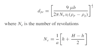
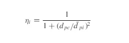
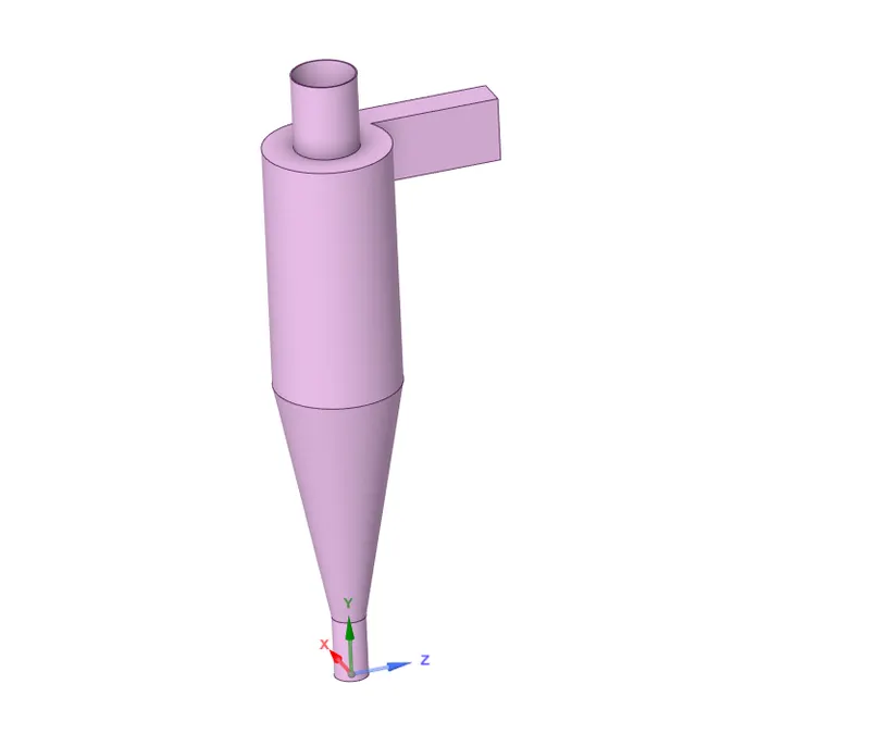
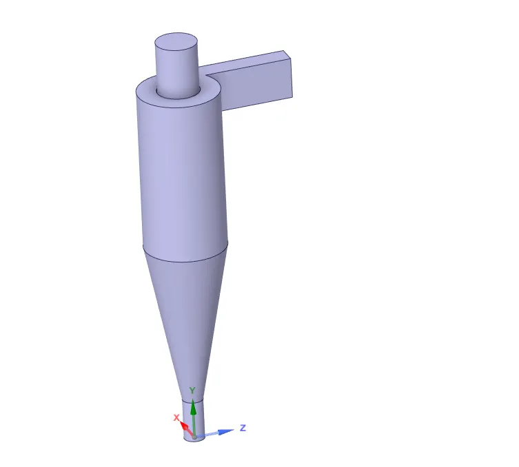
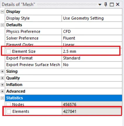
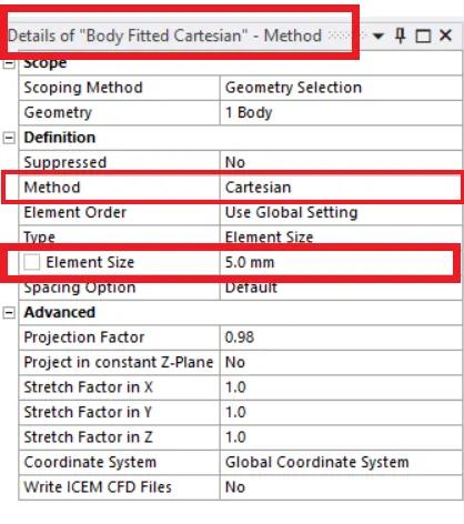
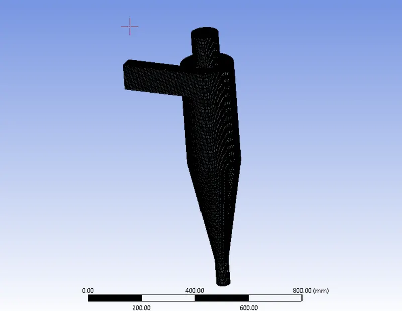
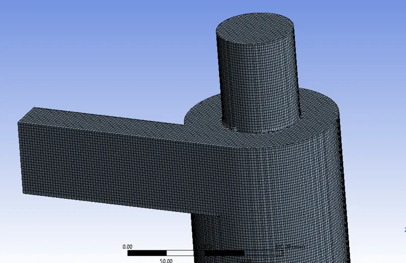
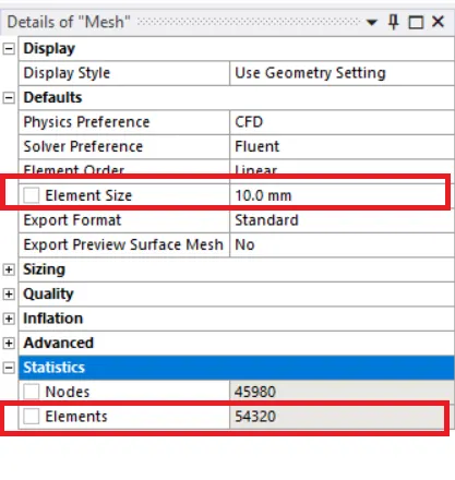
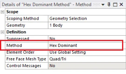
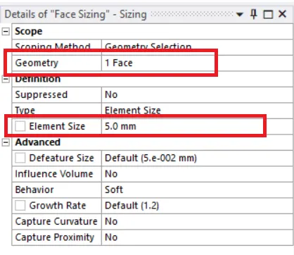
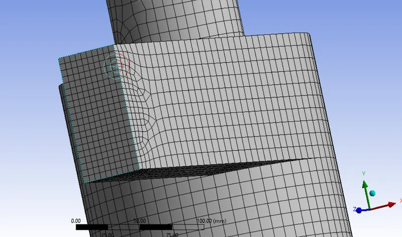
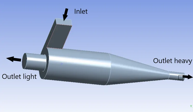
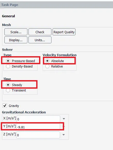
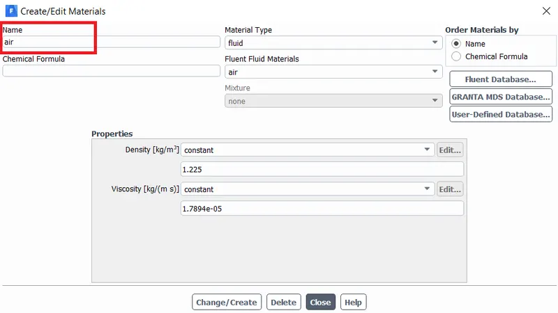
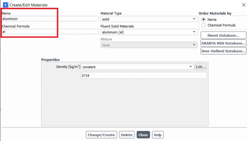
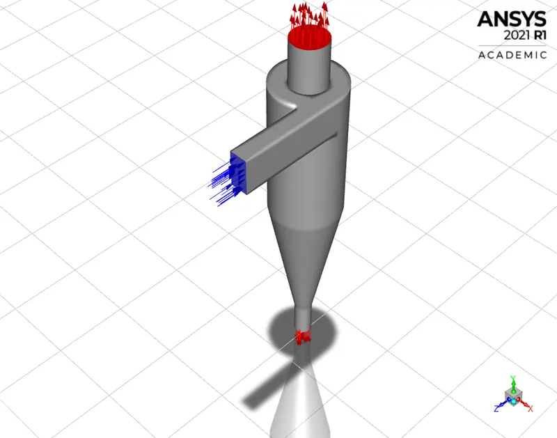
The general solver setting was set to pressure based with absolute velocity formulation and steady state solution .Gravity was set to 9.81 along -y direction . The working fluid was selected as air and material for seperator was chosen as Aluminium.
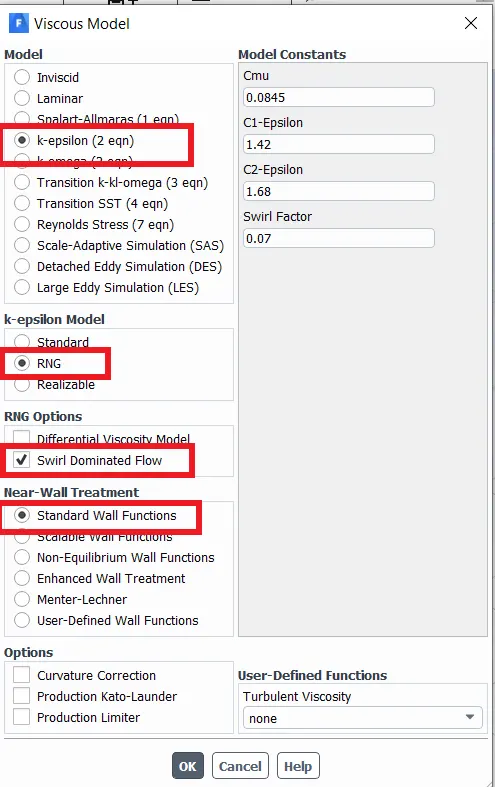
The viscous model was set to RNG k-epsilon with swirl dominated flow and standard wall functions.
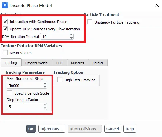
The Discrete Phase Modelling option was chosen with Anthracite as material , particle of size 1micrometer was chosen and was injected along inlet surface with velocity 3m/s .
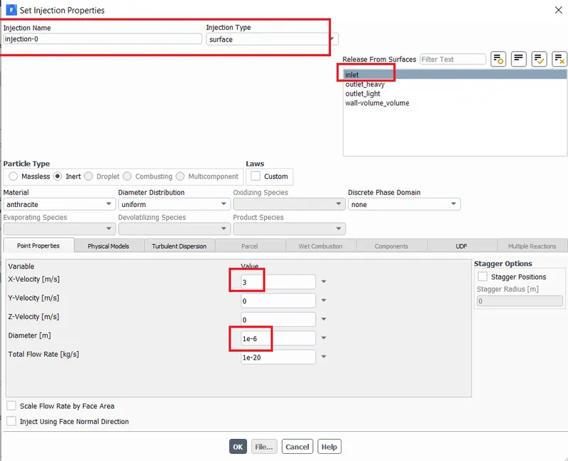
Boundary Conditions
Inlet :
Velocity =3 m/s
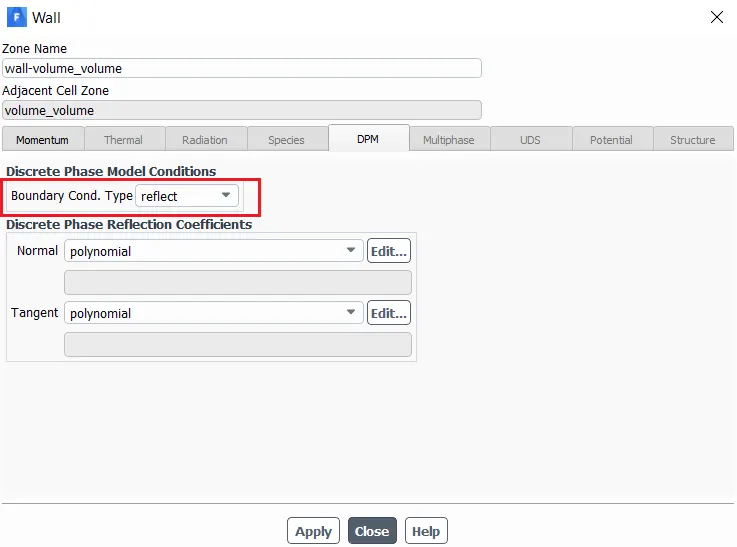
DPM phase type = Reflect
Outlet heavy :
DPM phase type = Trap
Outlet light :
DPM phase type = Escape
Wall :
DPM phase type = Reflect
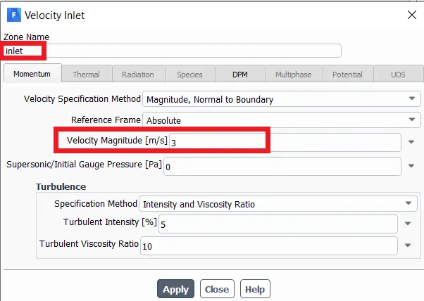
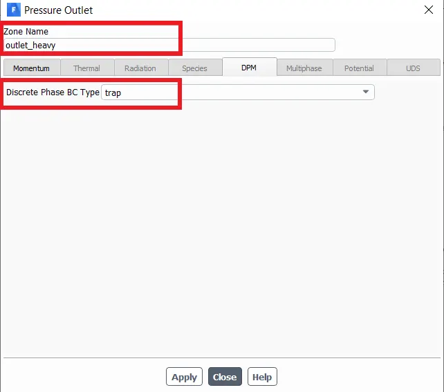
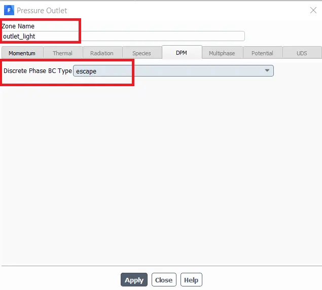
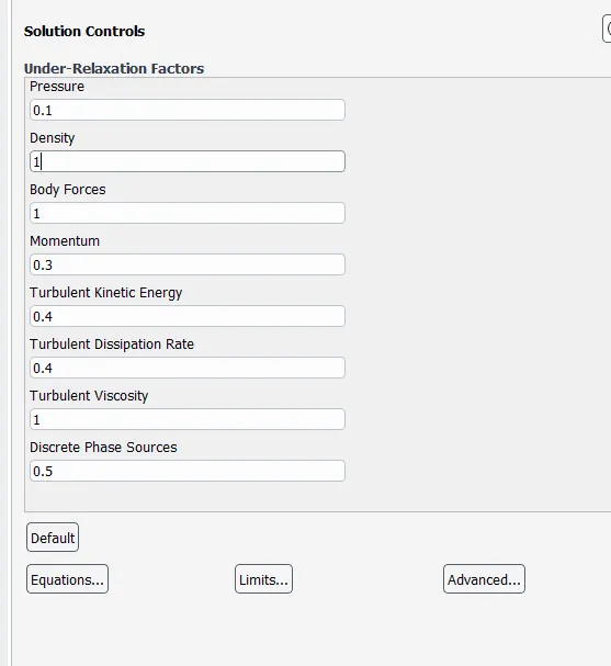
The under relaxation factors for solution controls were altered and momentum , turbulent kinetic energy and turbulent dissipation rate discretization was changed to First order upwind .
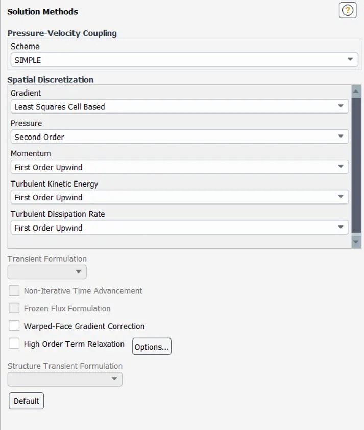
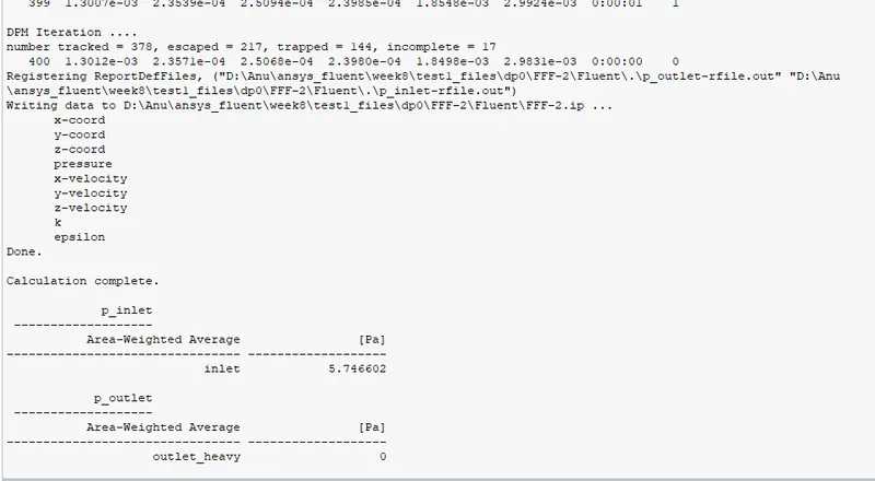
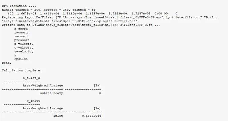
Report Definitions were requested for area weighted pressure calculation at inlet and outlet .
The solution was initialized using standard option with reference as inlet .
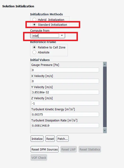
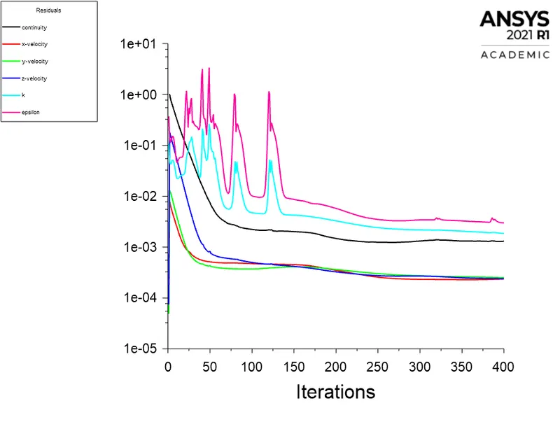
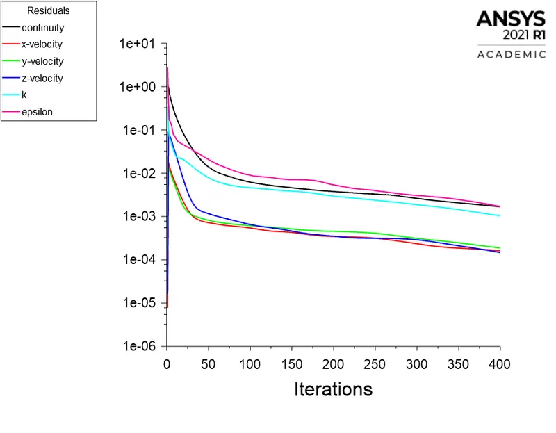
The solution was run for 400 Iterations
Results :
Case 1:
Particle size : 1 `mum`
inlet velocity : 3 m/s
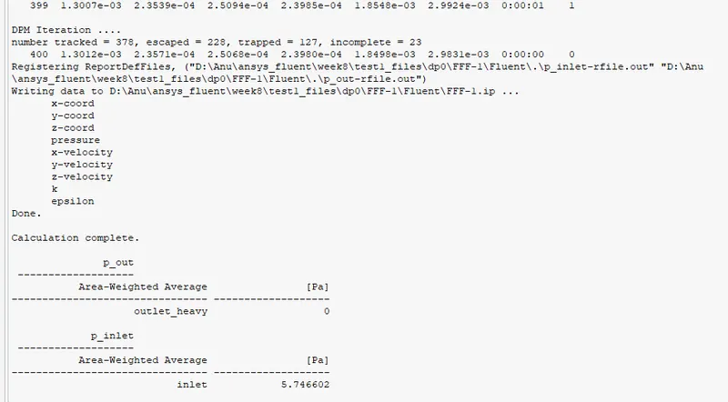
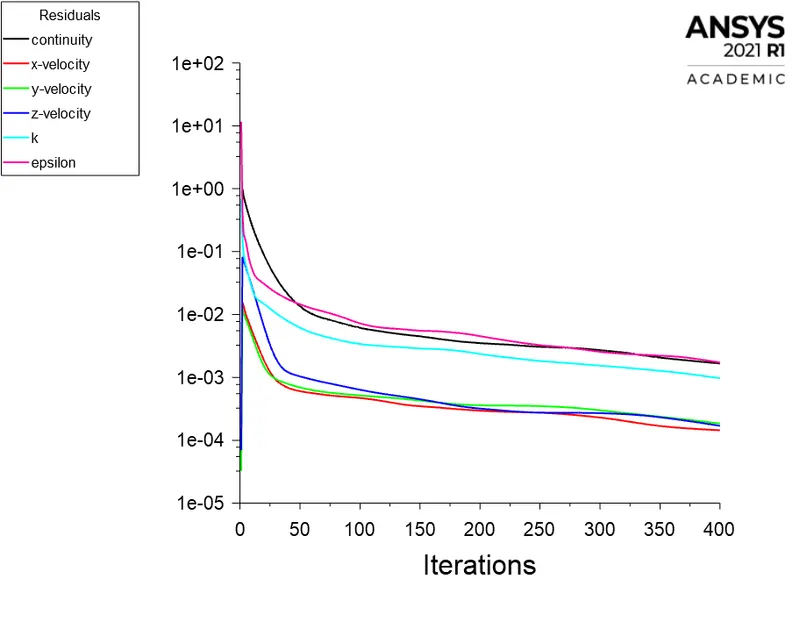
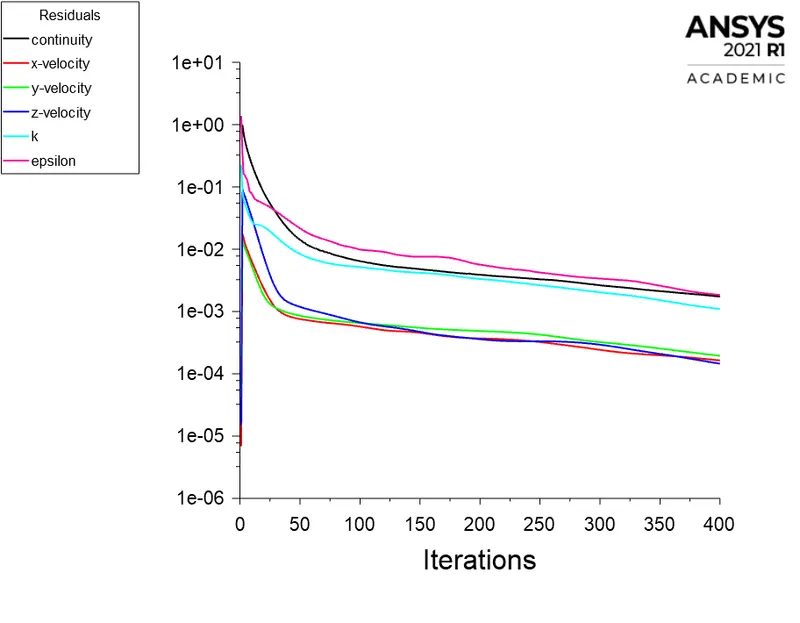
Scaled Residuals
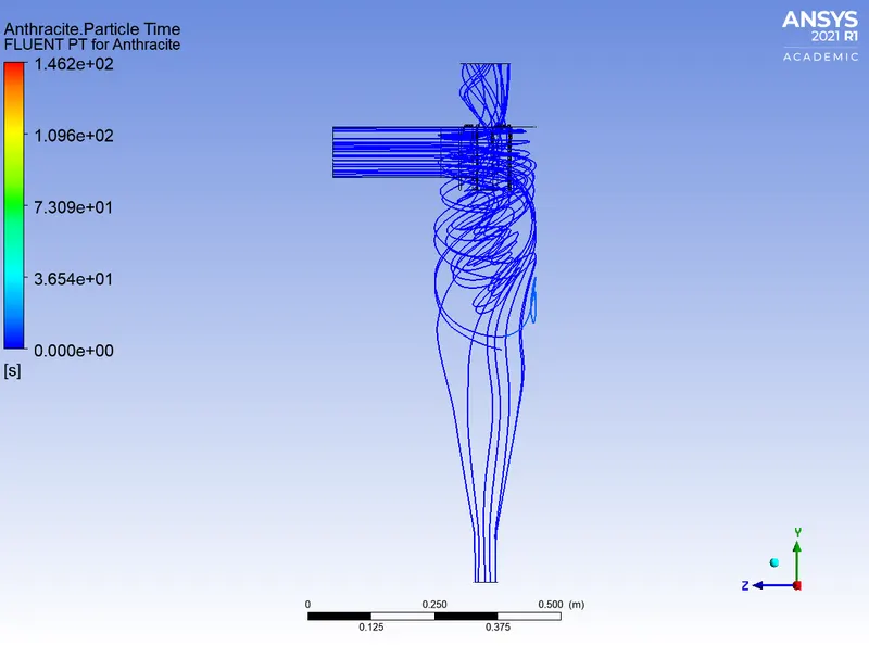
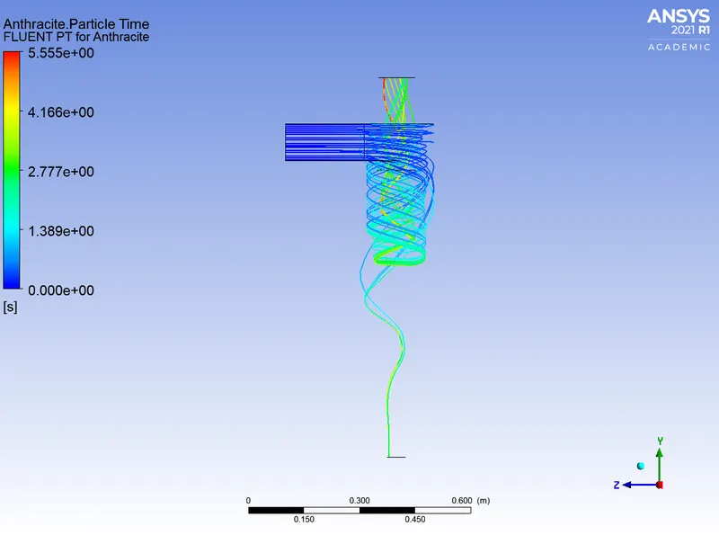
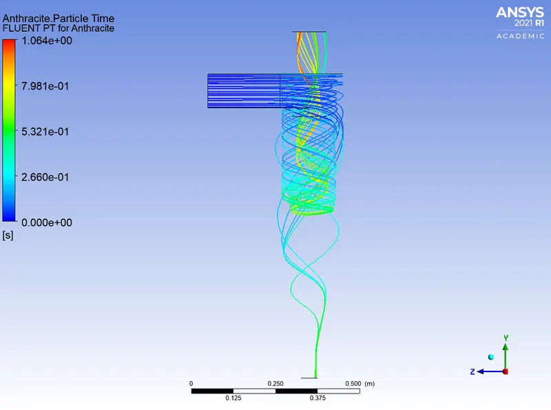
Particle Time Contour
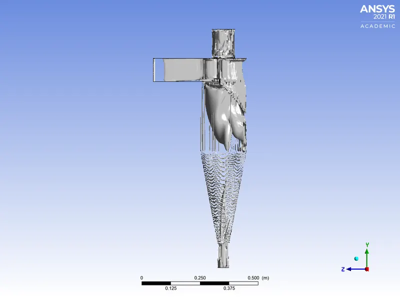
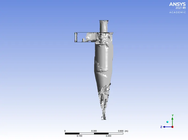
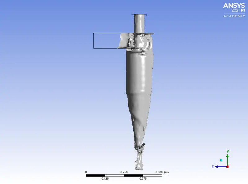
Vortex Region
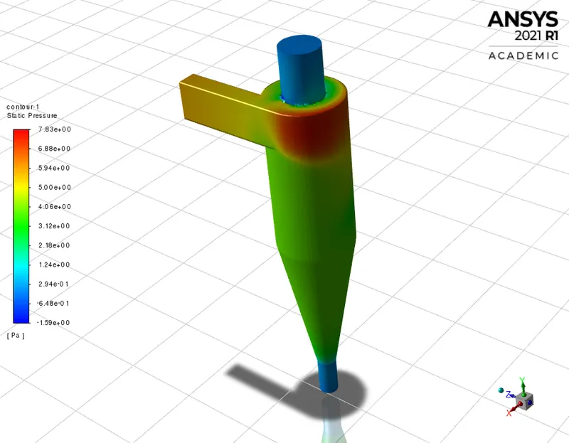
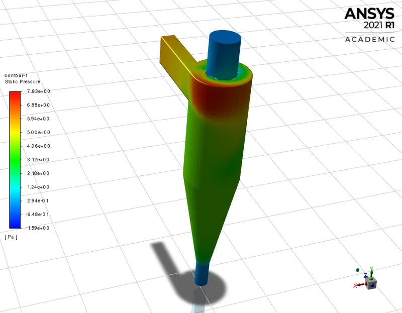
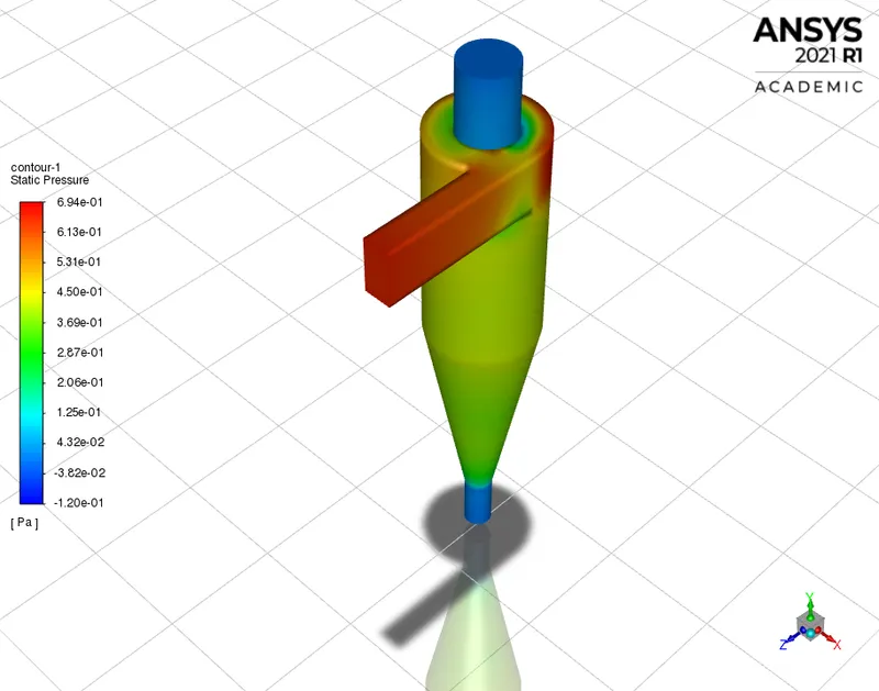
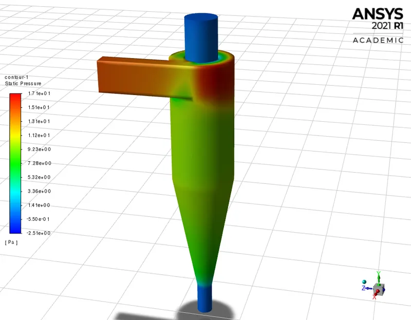
Pressure Contour
Case 2:
Particle size : 5 `mum`
inlet velocity : 3 m/s
Scaled Residuals
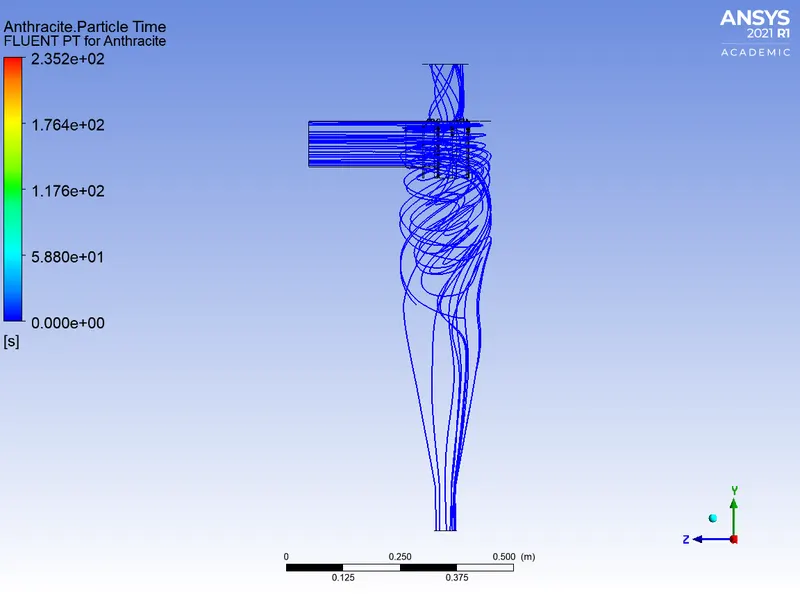
Particle Time Contour
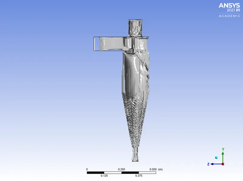
Vortex Region
Pressure Contour
Case 3:
Particle size : 5 `mum`
inlet velocity : 1 m/s
particle velocity : 1m/s
Scaled Residuals
Particle Time Contour
Vortex Region
Pressure Contour
Case 4:
Particle size : 5 `mum`
inlet velocity : 3 m/s
particle velocity : 1m/s
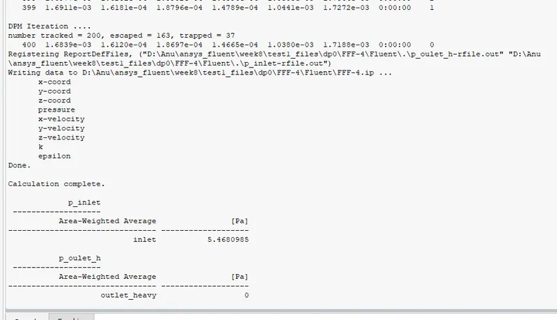
Scaled Residuals
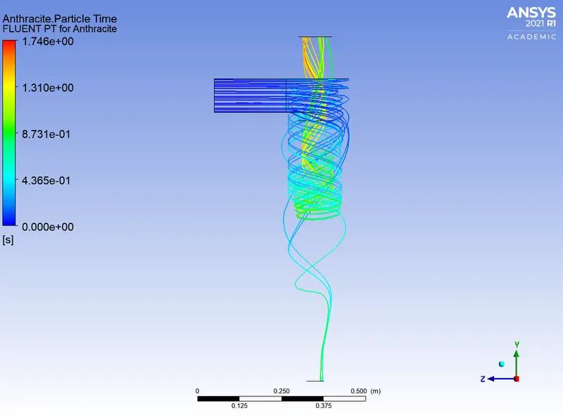
Particle Time Contour
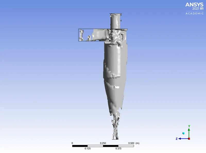
Vortex Region
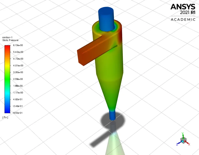
Pressure Contour
Case 5:
Particle size : 5 `mum`
inlet velocity : 5 m/s
particle velocity : 1m/s
Scaled Residuals
Particle Time Contour
Vortex Region
Pressure Contour
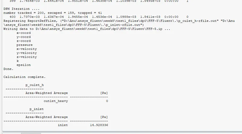
| Case no | Inlet Velocity (m/s) | Particle Size( `mum`) | Pressure drop (Pa) |
Efiiciency in % Trapped/Tracked |
| 1 | 3 | 1 | 5.74 | 33 .59 |
| 2 | 3 | 5 | 5.746 | 38.09 |
| 3 | 1 | 5 | 0.653 | 15.55 |
| 4 | 3 | 5 | 5.46 | 18.5 |
| 5 | 5 | 5 | 14.92 | 20.5 |
Inference
From the table , we can conclude that
1) As particle size increases , efficiency increases for a given inlet velocity .
2) As inlet velocity increases, pressure drop increases as well as efficiency increase for a given particle size.