Simulating Cyclone separator with Discrete Phase Modelling
AIM :
To perform analysis on cyclone separator and calculate the separation efficiency and pressure drop.
OBJECTIVE:
- Understand the any four empirical models used to calculate the cyclone separator efficiency.
- To perform an analysis on a given cyclone separator model by varying the particle diameter from 1 μm to 5 μm and calculate the separation efficiency in each case. Discuss the results. velocity = 3m/sec.
- To perform an analysis on a given cyclone separator model by varying the particle velocity from 1 m/sec to 5 m/sec and calculate the separation efficiency and pressure drop in each case. Discuss the results. particle diameter size = 5 μm also, the flow velocity same as particle velocity.
THEORY:
Cyclone separator
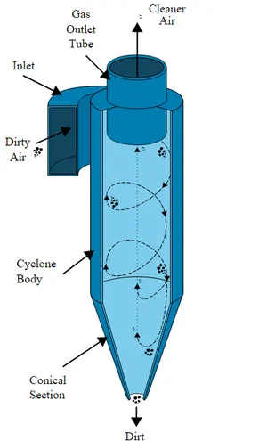
Working Principle
A cyclone is a centrifugal separator in which particles, due to their mass, are pushed to the outer edges as a result of centrifugal force. Incoming air is automatically forced to adopt a fast-revolving spiral movement - the so-called double vortex. This double spiral movement consists of an outer stream, which flows downwards in a spiral, and an inner stream, which flows upwards in a spiral. At the interchange between both streams, air passes from one stream to the other. The particles which are present in the air are forced to the outer edges and leave the separator via a collection device fitted to the bottom of the separator.
Materials
In the presence of substances and liquids with a strong corrosive or erosive nature, cyclones must be made of a suitable material or be coated with an appropriate substance. Cyclones are available in various materials such as stainless steel, aluminium, nickel, polystyrene (PS), polyvinylchloride (PVC) and polyvinylidenefluoride (PVDF).
Application
Wood and furniture industry
The building sector
Glass industry
The transport sector for storage and transfer
The foodstuffs industry
Waste combustion installations
The chemicals industry.
Empirical models used for cyclone separator efficiency
1.Iozia and Leith Model
Iozia and Leith logistic model is a modified version of Barth Model, which is developed based on force balance.The model assumes that a particle carried by the vortex endures the influence of two forces: a centrifugal force, Z and a flow resistance, W. The collection efficiency & `eta_i` of particle diameter dpi can be calculated from
`eta_i = 1/{1+(d_(pc)/d_(pI))^beta}`
`beta` is an expression for slope parameter derived based on the statistical analysis of experimental data of a cyclone with D =0.25 m given as
`beta = 0.62-0.87ln(d_{pc}/100)+5.21ln({ab}/D^2)+1.05[ln((ab)/D^2)]^2`
`d_{pI} =`Particle diameter.
`d_{pc} =`50% cut size given by Barth.
2.Li and Wang Model
The Li and Wang model includes particle bounce or reentrainment and turbulent diffusion at the cyclone wall. A twodimensional analytical expression of particle distribution in the cyclone is obtained. Li and Wang model was developed based on the following assumptions
- The radial particle velocity and the radial concentration profile are not constant for uncollected particles within the cyclone.
- Boundary conditions with the consideration of turbulent diffusion coefficient and particle bounce reentrainment on the cyclone wall are
C = `C_0`, at `theta =0`
`Dr {delC}/{del r} = (1-alpha)omegac`, at r = D/2
The tangential velocity is related to the radius of cyclone by `uR^n` = constant.
The resultant expression of the collection efficiency for particle of any size is given as
`eta_i = 1- exp{-lambdatheta_1}`
where,
`theta_1 = 2pi(S+L)/a`
3.Koch and Licht Model
Koch and Licht collection theory recognized the inherently turbulent nature of cyclones and the distribution of gas residence times within the cyclone. Koch and Licht described particle motion in the entry and collection regions with the additional following assumptions:
- The tangential velocity of a particle is equal to the tangential velocity of the gas flow, i.e. there is no slip in the tangential direction between the particle and the gas.
- The tangential velocity is related to the radius of cyclone by `uR^n`= constant.
A force balance and an equation on the particles collection yields the grade efficiency `eta_i`
`eta_i = 1- exp{-2[[Gtau_iQ]/D^3(n+1)]^(0.5/(n+1)}}`
where,
`G ={8K_c}/(K_a^2K_b^2)`
`eta = 1 - {1 - ((12D)^0.14)/2.5}{(T+460)/530}^0.3`
`tau_i = {rho_pd_(pI)^2}/{18mu}`
G is a factor related to the configuration of the cyclone, n is related to the vortex and `tau` is the relaxation term
4.Lapple Model
Lapple model was developed based on force balance without considering the flow resistance. Lapple assumed that a particle entering the cyclone is evenly distributed across the inlet opening. The particle that travels from inlet half width to the wall in the cyclone is collected with 50% efficiency. The semiempirical relationship developed by Lapple to calculate a 50% cut diameter, dpc, is
`d_(pc)=[{9mub}/{2piN_ev_i(rho_p-rho_g)}]^(1/2)`
where Ne is the number of revolutions
`N_e = 1/a[h+{H-h}/2]`
The efficiency of collection of any size of particle is given by
`eta_i = 1/(1+(d_(pc)/d_(pI))^2)`
BODY OF THE CONTENT:
Geometry preparation
For this project the geometry was already prepared using a CAD package. The geometry can be found here.
we open an empty fluent module and import the geometry onto spaceclaim.
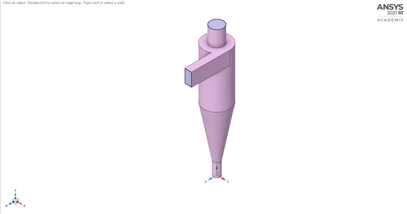
From this geometry we extract the fluid volume using the volume extract option in the prepare tab. We select the openings and the fluid volume will be extracted which is as shown
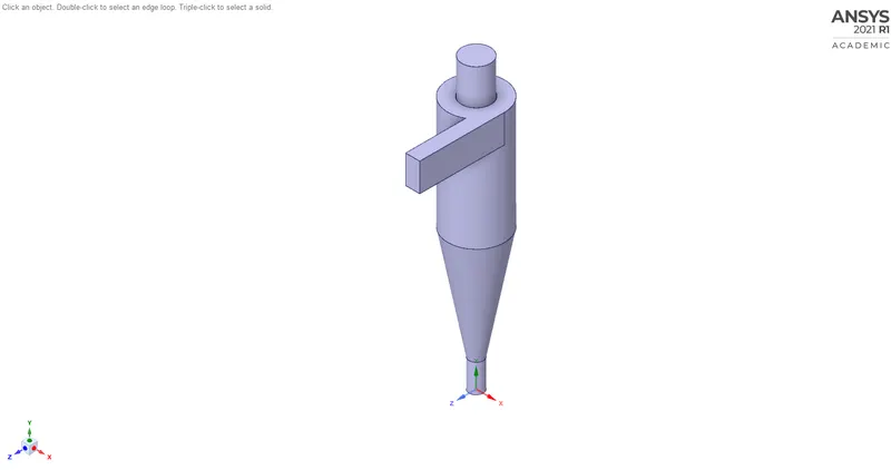
we suppress the outer volume using the suppress for physics option and close the spaceclaim module. This geometry will be updated onto fluent workbench.
Meshing
Before meshing the geometry we first create named selections
we name the inlet and outlets as follows.
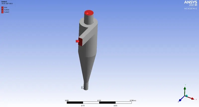
Next we give the mesh sizing as 1e-2m. Mesh sizing is important as it determines how many particles enter through the inlet. The number of cells on the inlet is the number of particles entering through the inlet.
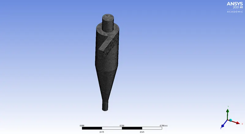
we close this meshing module and update the ansys workbench so that the meshing gets updated onto the workbench.
Case Setup
For this case we choose a steady state, pressure based solver. we give gravity in the -y direction as 9.81 m/s^2. The viscous model for this will be RNG K-`epsilon` with swirl dominated flow. For modeling the solid particles we use DPM (Discrete Phase Modeling) with the following inputs
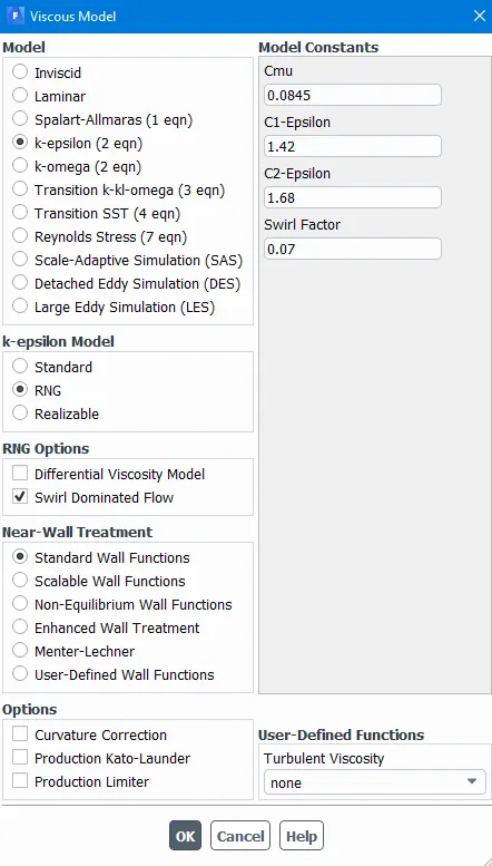
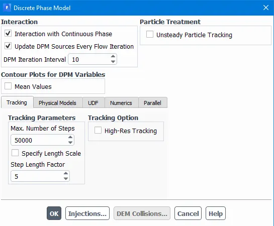
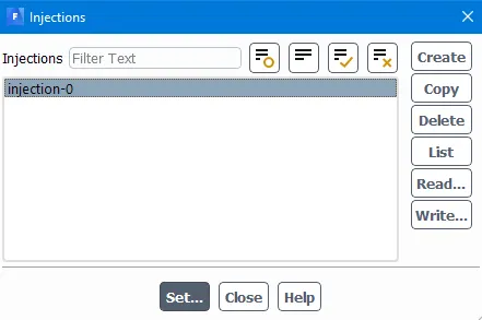
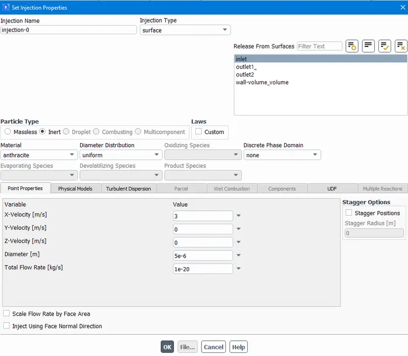
The BCs are as follows
Inlet and wall :- Reflect with the inlet velocity being the same as the particle inlet velocity which is 3m/s. This velocity will be changed to see the effects of velocity over the efficiency of the cyclone seperator.
Outlet(Top):-Escape
Outlet(Bottom/dustbin) - Trap
In the methods we select the following options.
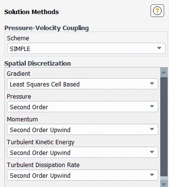
Now we initialise the solution as follows
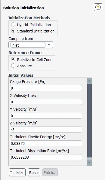
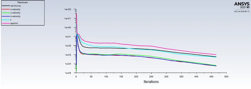
Once the initialisation is done we give the number of iterations as 600 and run the simulation for different cases such as
- Diameter from 1 `mum` to 5 `mum` with velocity 3m/sec
- Particle velocity as 1m/s to 3 m/s with particle diameter 5 `mum`
we get the following results.
RESULTS
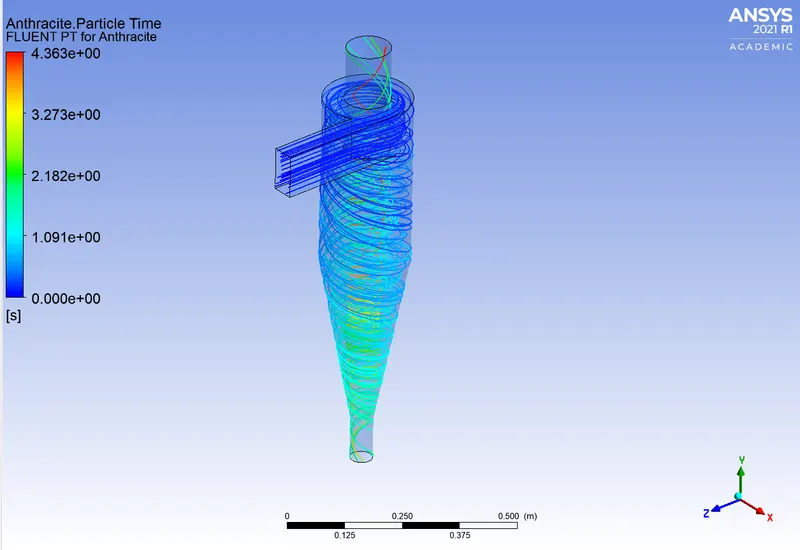
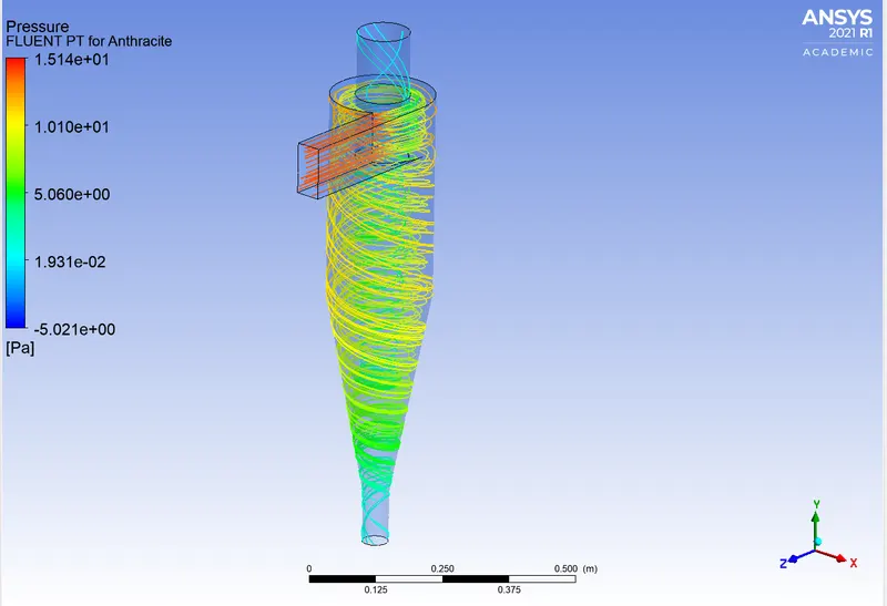
1 `mum`, velocity 3m/s
Residual plot
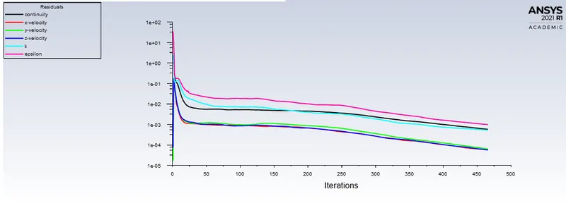
Console output

The cyclone seperator efficiency is given by the ratio of no of particles trapped to the number of particles tracked.
`eta` = `27/124*100 = 21.77%`
Contour
Pressure
Video animation
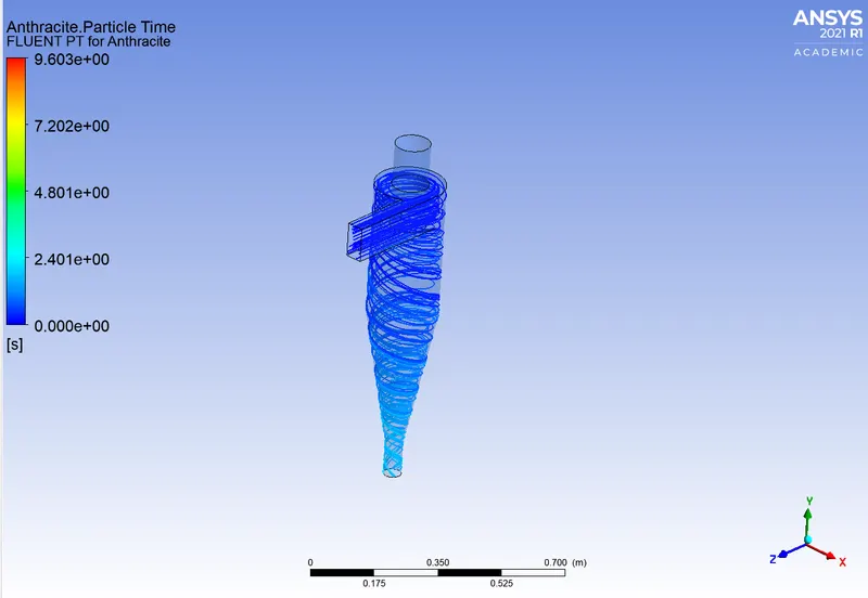
5 `mum`, velocity 3m/s
Residual plot
Console output

The cyclone seperator efficiency is given by the ratio of no of particles trapped to the number of particles tracked.
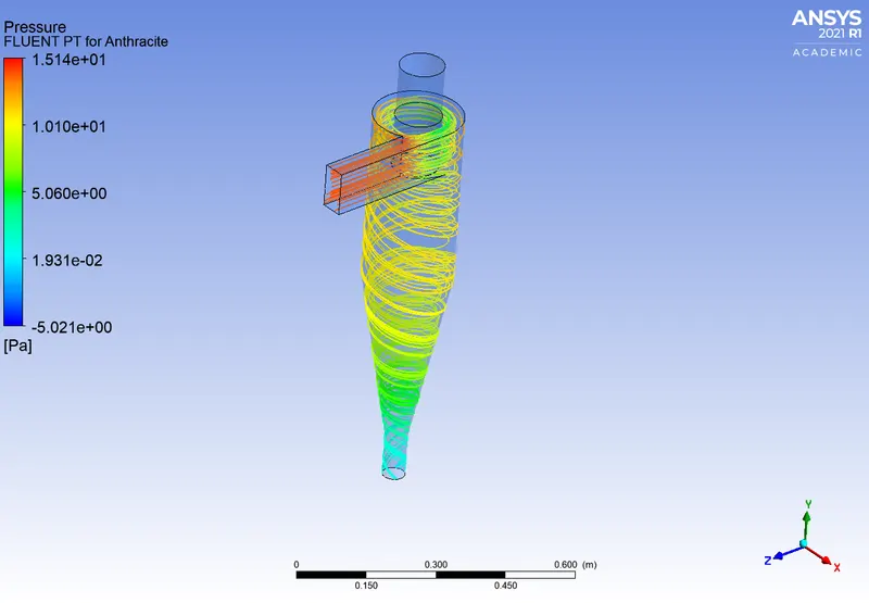
`eta` = `119/124*100 = 95.96%`
Contour
Pressure
Video animation
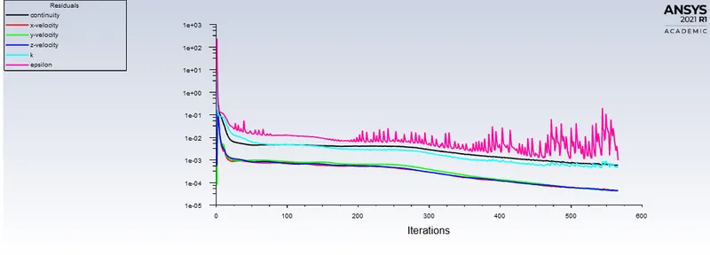
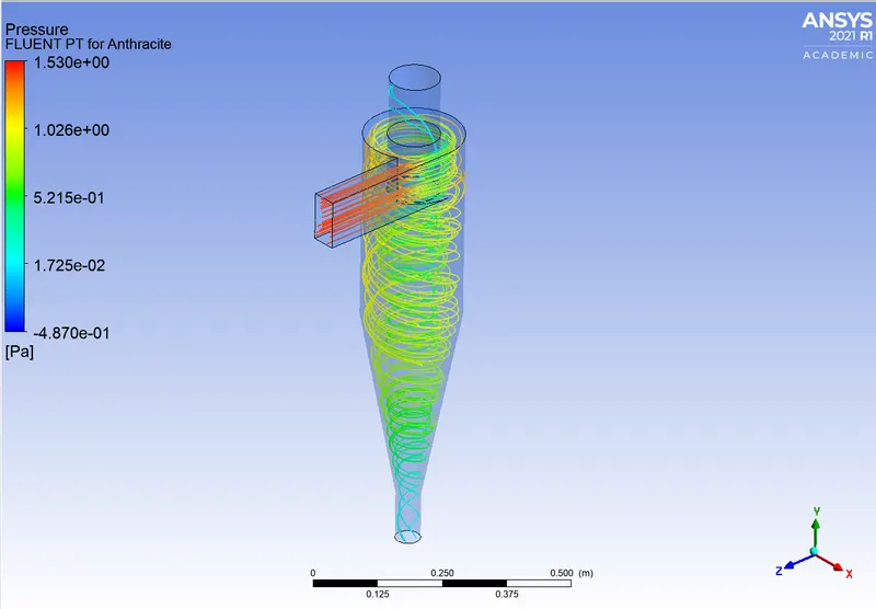
5 `mum`, velocity 1m/s
Residual plot
Console output

The cyclone seperator efficiency is given by the ratio of no of particles trapped to the number of particles tracked.
`eta` = `10/124*100 = 8%`
Contour
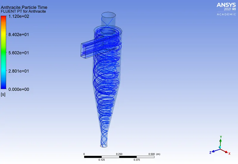
Pressure
Video animation
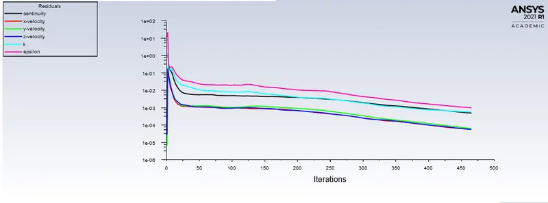
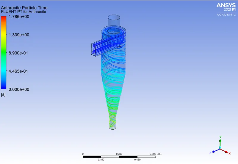
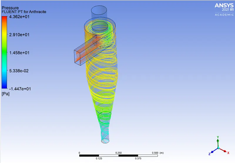
5 `mum`, velocity 5m/s
Residual plot
Console output

The cyclone seperator efficiency is given by the ratio of no of particles trapped to the number of particles tracked.
`eta` = `123/124*100 = 99.19%`
Contour
Pressure
Video animation
| Size (micrometers) | Velocity (m/s) | Efficiency (%) | Pressure drop (Pa) (in-ou) |
| 1 | 3 | 21.77 | 20 |
| 5 | 3 | 95.96 | 20 |
| 5 | 1 | 8 | 2 |
| 5 | 5 | 99.19 | 57 |
CONCLUSION:
From the above results it is observed that
- As the size of the particle increases the efficiency also increases
- For the same particle size as the velocity of the particle increases the efficiency of the particle increases and the pressure drop of the particle also increases due to inertia.