Week 8 - Simulating Cyclone separator with Discrete Phase Modelling

Aim: - To perform analysis on cyclone separator and calculate the separation efficiency and pressure drop.

Objective: -

1. To discuss about four empirical models used to calculate the cyclone separator efficiency.
2. To perform an analysis on a given cyclone separator model by varying the particle diameter from 1 μm to 5 μm and calculate the separation efficiency for each case.
3. To perform an analysis on a given cyclone separator model by varying the particle velocity from 1 m/sec to 5 m/sec using particle diameter of 5 μm and calculate the separation efficiency and pressure drop in each case.

Theory: -

Cyclone Separator –

These are separation devices that use the principle of inertia to remove particulate matter from flue gases. Cyclone separator is one of many air pollution control devices known as pre-cleaners since they generally remove larger pieces of particulate matter.

It works much like a centrifuge, but with a continuous feed of flue gases and air. In it, dirty flue gas is fed into a chamber. The inside of the chamber creates a spiral vortex, similar to a tornado. The lighter components of this gas have less inertia, so it is easier for them to be influenced by the vortex and travel up it. Contrarily, larger components of particulate matter have more inertia and are not as easily influenced by the vortex.

These can vary drastically in their size. The size of the cyclone depends largely on how much flue gas must be filtered; thus, larger operations tend to need larger cyclones. it can range from a relatively small 1.21.5 meters tall (about 4-5 feet) to around 9 meters (30 feet)—which is about as tall as a three-story building.

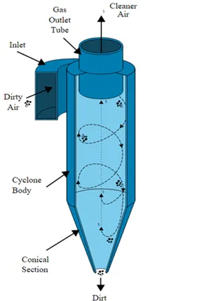
Cyclone Efficiency Empirical Models–

• Iozia and Leith Model:

Iozia and Leith logistic Model is a modified version of Barth (1956) model which is developed based on force balance. The model assumes that a particle carried by the vortex endures the influence of two forces: a centrifugal force Z, and flow resistance, W. The collection efficiency of particle diameter dpi can be calculated by

`η_i =1/(1 +(d_(pc)/d_(p i ))^β )`

where β is an expression for slope parameter derived based on the statistical analysis of experimental data of a cyclone with D =0.25 m and dpc is the 50% cut size given by Barth

`dpc = ((9µQ)/(πρp z_c v_(t max)^2 ))^0.5` , where core length zc, and core diameter dc.

• Li and Wang Model:

The Li and Wang model include particle bounce or re-entrainment and turbulent diffusion at the cyclone wall. A two-dimensional analytical expression of particle distribution in the cyclone is obtained. Li and Wang model was developed based on the following assumptions:

1.The radial particle velocity and the radial concentration profile are not constant, for uncollected particles within the cyclones.

2.Boundary conditions with the consideration of turbulent diffusion coefficient and particle bounce re-entrainment on the cyclone wall are:

c = c₀ at θ = 0

D_r (∂c/∂r) = (1 − α) wc at r = D/2

3.The tangential velocity is related to the radius of cyclone by: u*Rn = constant.

The expression of the collection efficiency for particle of any size is given as

η_i = 1 − exp{−λθ₁}

where θ₁ = 2π (S + L)/a and λ = (1 − α) K w_w / D_r r_wⁿ

• Koch and Licht Model:

Koch and Licht collection theory recognized the inherently turbulent nature of cyclones and the distribution of gas residence times within the cyclone. Koch and Licht describe particle motion in the entry and collection regions with the additional following assumptions:

1.The tangential velocity of a particle is equal to the tangential velocity of the gas flow i.e., there is no slip in the tangential direction between the particle and the gas.

2.The tangential velocity is related to the radius of cyclone by: u*Rn = constant.

The expression or efficiency is given by –

ηi = 1 – exp [−2 [(Gτ_iQ/D³) (n + 1)]^0.5/(n+1)

• Lapple Model:

Lapple model was developed based on force balance without considering the flow resistance. Lapple assumed that a particle entering the cyclone is evenly distributed across the inlet opening. The particle that travels from inlet half-width to the wall in the cyclone is collected with 50% efficiency. The semi-empirical relationship developed by Lapple to calculate a 50% cut diameter d_pc is

`dpc =[(9µb)/(2π N_(e) v_i (ρ_p - ρg) )]^(1/2)` , where N_e is the number of revolutions.

The efficiency of collection of any size of particle is given by:

`η_i=1/( 1 + (d_(pc)/d_(p i) )^2 )`

Applications:

1. Chemical and Petrochemical Processes
2. Industrial, Metallurgical and Power Generation
3. Food & Pharmaceutical
4. Cement Industry

Case Setup: -

Geometry – Fluid volume is extracted from the given Cyclone separator Model in SpaceClaim. The model is then suppressed for physic and fluid volume is used for further analysis.

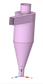
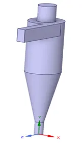
Cyclone separator Model Extracted Fluid Volume

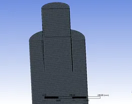
Meshing –

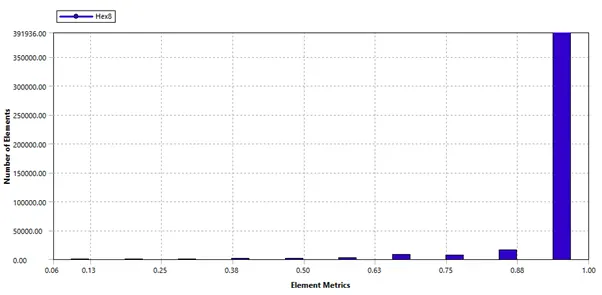
Element size = 5mm No. of Nodes = 4,56,576 No. of Elements = 4,27,841

Method = Body fitted Cartesian

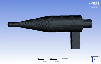
Element Quality

Fluent setup:

• Pressure based solver and Absolute velocity is used.
• Steady-state Calculation is performed.
• Gravity is enabled in -ve Y axis.
• K-ɛ RNG model is used with swirl dominating flow option marked.
• Discreate Phase Modeling Option is enabled and size and velocity is modified to suit each case.
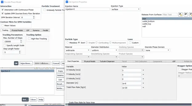
• Inlet velocity is set according to each case.
• DPM option in boundary condition set as – Inlet and wall: - Reflect

  Outlet_Top: - Escape

  Outlet_Bottom: - Trap

Two cases are used to study the cyclone separator

1. Varying size with inlet/particle velocity equal to 3m/s.
2. particle size 5 µm with varying inlet/particle velocity 1m/s - 5 m/s.

Case A. Varying Size (1-5 µm) with inlet velocity 3m/s

1. Size 1 µm

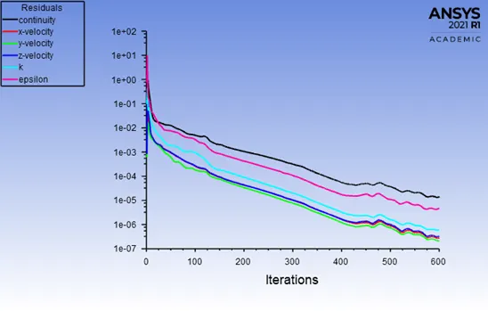
Residue Plot:

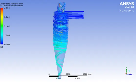
Residence time:

Particle tracking:

Separation efficiency = No. of particle Trapped/No. of Particle Tracked = 209/378 = .5529

2. Size 2 µm

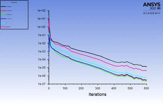
Residue Plot:

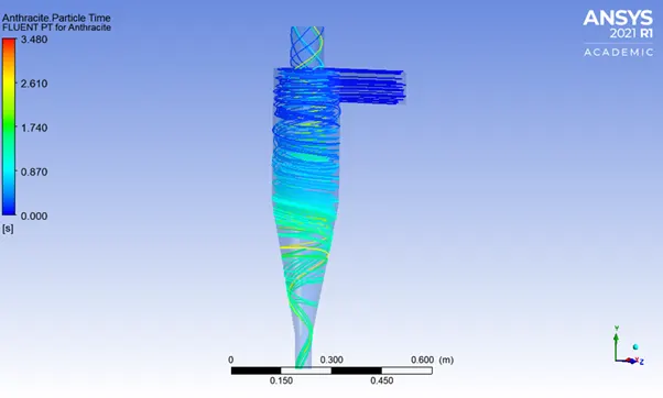
Residence time:

Particle tracking:

Separation efficiency = No. of particle Trapped/No. of Particle Tracked = 244/378 = .6455

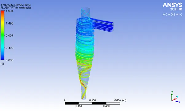
3. Size 3 µm

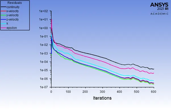
Residue Plot:

Residence time:

Particle tracking:

Separation efficiency = No. of particle Trapped/No. of Particle Tracked = 270/378 = .7143

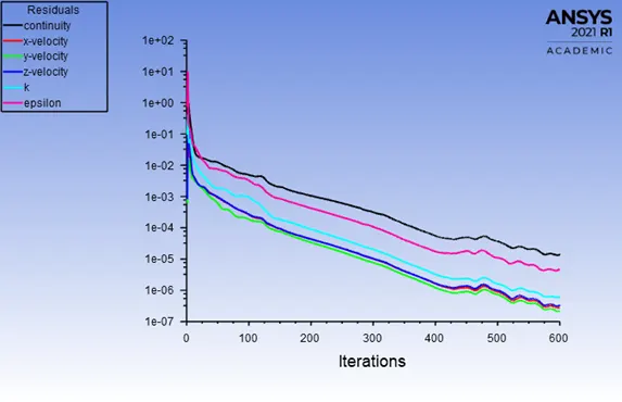
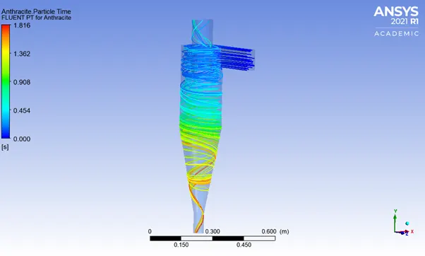
4. Size 4 µm

Residue Plot:

Residence time:

Particle tracking:

Separation efficiency = No. of particle Trapped/No. of Particle Tracked = 294/378 = .7778

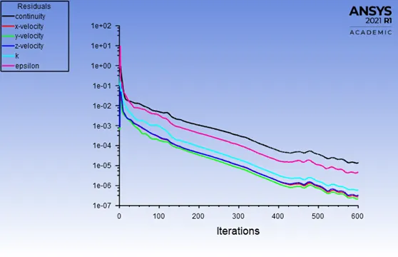
5. Size 5 µm

Residue Plot:

Residence time:

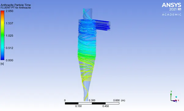
Particle tracking:

Separation efficiency = No. of particle Trapped/No. of Particle Tracked = 305/378 = .8068

Case B. Particle size 5 µm with varying inlet/particle velocity 1m/s - 5 m/s.

1. inlet Velocity = 1m/s

Residue Plot:

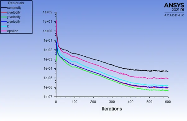
Residence time: Pressure Contour:

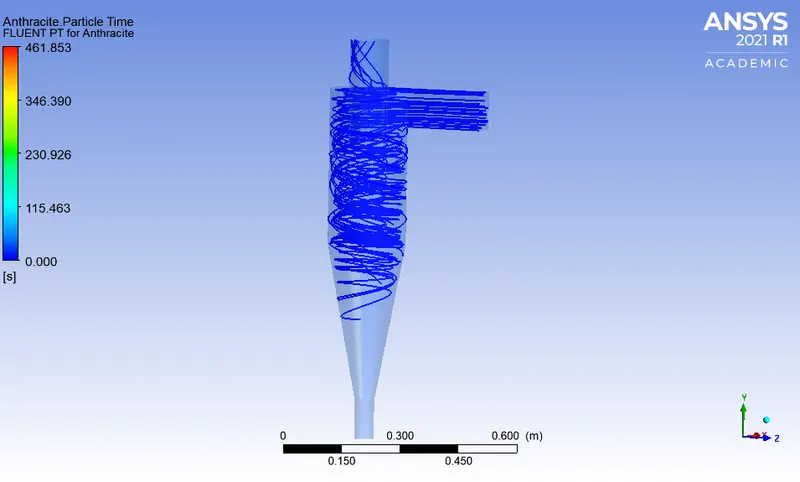
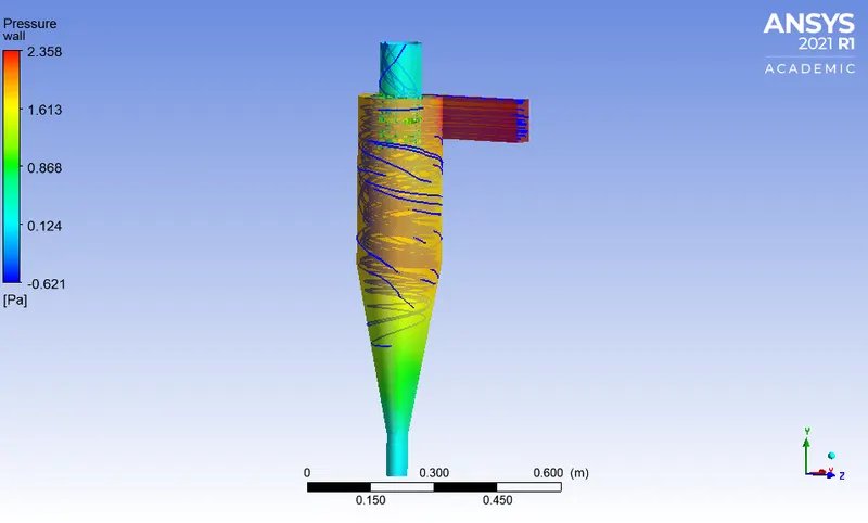
Particle tracking:

Separation efficiency = No. of particle Trapped/No. of Particle Tracked = 1/378 = 0.0026

2. inlet Velocity = 2m/s

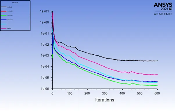
Residue Plot:

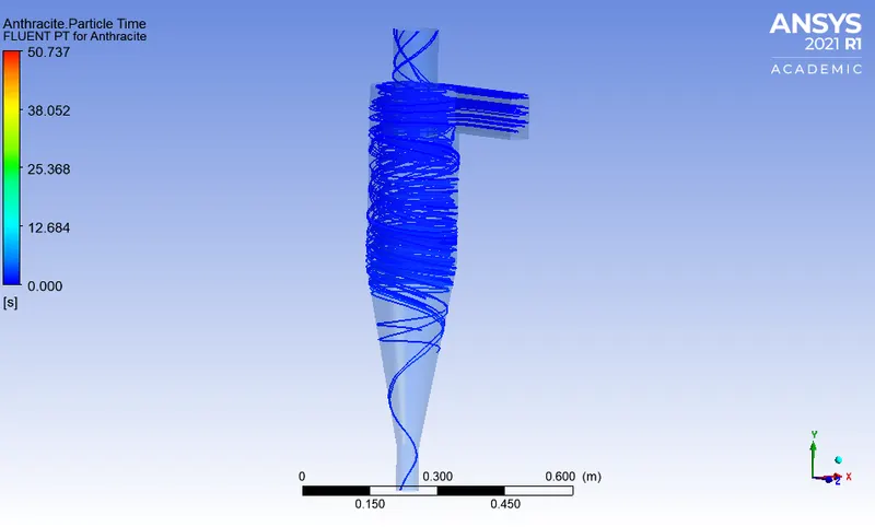
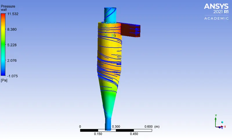
Residence time: Pressure Contour:

Particle tracking:

Separation efficiency = No. of particle Trapped/No. of Particle Tracked =71 /378 = 0.1878

3. inlet Velocity = 3 m/s (same as of Case A: 5)

Residue Plot:

Residence time: Pressure Contour:

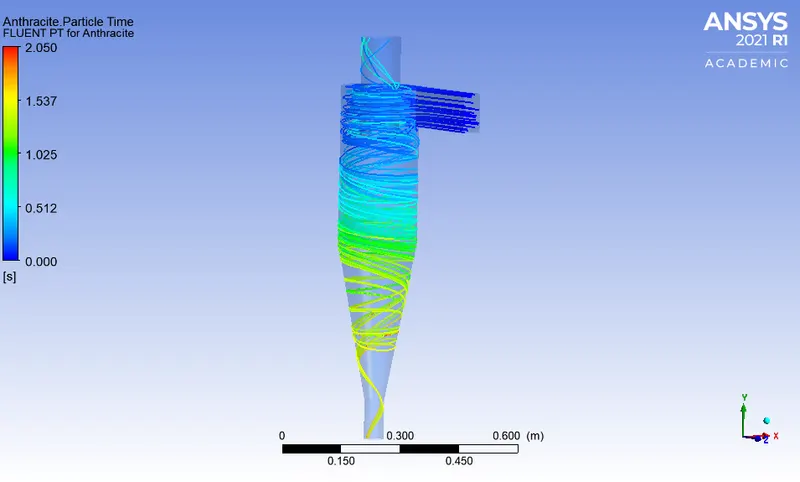
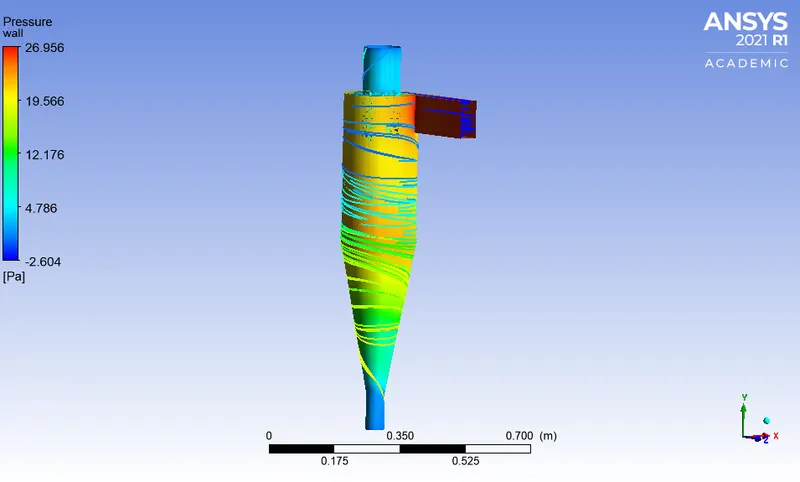
Particle tracking:

Separation efficiency = No. of particle Trapped/No. of Particle Tracked = 305/378 = .8068

4. inlet Velocity = 4m/s

Residue Plot:

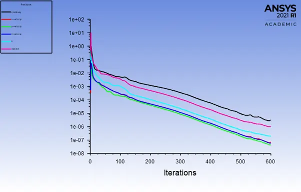
Residence time: Pressure Contour:

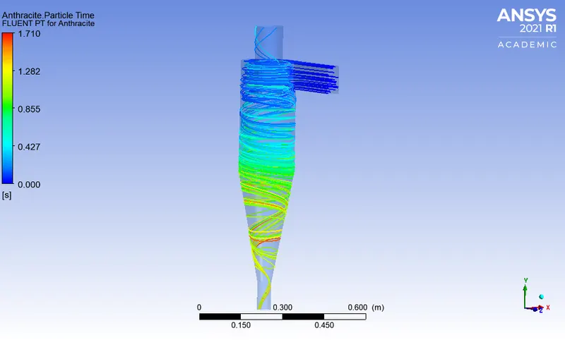
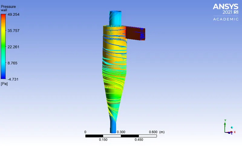
Particle tracking:

Separation efficiency = No. of particle Trapped/No. of Particle Tracked = 314/378 = 0.8306

5. inlet Velocity = 5m/s

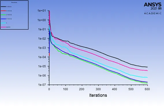
Residue Plot:

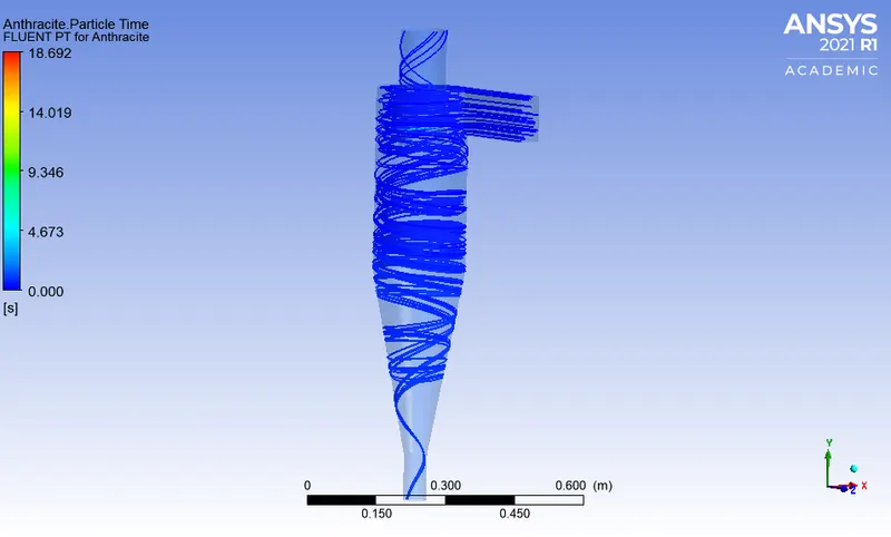
Residence time: Pressure Contour:

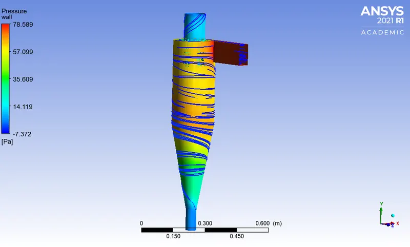
Particle tracking:

Separation efficiency = No. of particle Trapped/No. of Particle Tracked = 285/378 = 0.7540

Results: -

Case A: Varying size with inlet/particle velocity 3 m/s.

Particle Diameter	Particle Tracked	Particle Escaped	Particle Trapped	Incomplete	Separation Efficiency
1 µm	378	149	209	20	55.29 %
2 µm	378	133	244	1	64.55 %
3 µm	378	101	270	7	71.42 %
4 µm	378	77	294	7	77.78 %
5 µm	378	73	305	0	80.68 %

As the diameter tends to increase the particles become heavier and thus tend to settle down at Outlet_ Bottom (Trapped). The finer/ lighter Particles tends to escape from Outlet_Top. Hence as Size increase separation efficiency tends to increase.

Case B: Particle Size = 5 µm varying Inlet/Particle velocity

Particle velocity	Particle Tracked	Particle Escaped	Particle Trapped	Incomplete	Separation Efficiency	Pressure Drop (Pa)
1 m/s	378	97	1	280	0.26 %	2.979
2 m/s	378	75	71	232	18.78 %	12.607
3 m/s	378	73	295	6	78.04 %	29.56
4 m/s	378	64	314	0	83.06 %	53.985
5 m/s	378	74	285	19	75.40 %	85.961

As velocity tends to increase the Pressure drop across inlet and Outlet increases. At lower velocities the particles are caught into recirculation zones and hence the tracking is dumped after 1,50,000 iterations, as more particles shows incomplete status, But as velocity increases the efficiency tends to increase giving best results at 4m/s and then tends to dip.