Project 2 - Rankine cycle Simulator

Aim: - To write a program in MATLAB to simulate Rankine cycle.

Objective: - 1. To calculate the state points for the Rankine cycle based on user inputs using XSteam.m file for steam table.

2. To plot the T-S and H-S curve for Rankine cycle.
3. To calculate work and heat exchange as well as other working parameters.

Theory: - The Rankine cycle is the fundamental operating cycle of all power plants where an operating fluid is continuously evaporated and condensed. It is an idealized thermodynamic cycle of a heat engine that converts heat into mechanical work while undergoing phase change. It is an idealized cycle in which friction losses in each of the four components are neglected. The heat is supplied externally to a closed loop, which usually uses water as the working fluid.

It consists of mainly four processes, which are as follow:

1. Process 1–2: Isentropic Expansion in turbine i.e. steam enters in turbine and expands resulting in work output which can be further used to generate electricity or other purposes.
2. Process 2–3: constant pressure heat rejection in condenser i.e. steam reject heat and undergo phase change to liquid.
3. Process 3–4: Isentropic compression by pump i.e. liquid is pumped isentropically from low pressure to high pressure. It requires somework input.
4. Process 4–5-6-1: constant pressure heat addition in boiler i.e. heat is added so as to convert liquid into steam by adding heat through combustion of fuel.

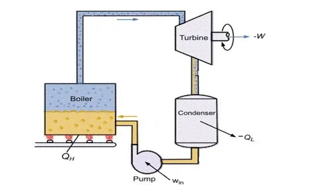
Some formulas used in calculations: -

heat input(qin) = h1−h4 heat output(qout) = h2−h3

work output by turbine(wt) = h1−h2 work input on pump (wp) = h4−h3

Net work output(wnet) = wt–wp Thermal efficiency(eff) = wnet/qin

back work ratio(bwr) = wp/wt specific steam consumption(ssc) = 3600/wnet

MATLAB code:-

close all
clear all
clc

%displaying the process involved
fprintf('%40s\n','RANKINE CYCLE SIMULATOR');
fprintf('\n1-2 is Isentropic Expansion in the turbine');
fprintf('\n2-3 is Constant Pressure Heat Rejection by the Condensor');
fprintf('\n3-4 is Isentropic Compression in the Pump');
fprintf('\n4-1 is Constant Pressure Heat Addition by the Boiler \n \n');

%asking for user inputs
p1=input('Enter the inlet pressure at turbine in bar:');
t1=input('Enter the inlet temperature at turbine in deg. celcius:');
p2=input('Enter the inlet pressure at condensor in bar:');

fprintf('\n%30s','RESULT');

p4=p1;
p3=p2;
%for 1st state
tsat1=XSteam('Tsat_p',p1);
sg1=XSteam('sV_p',p1);
hg1=XSteam('hV_p',p1);
cp1=XSteam('CpV_p',p1);
s1=XSteam('s_pT',p1,t1);
h1=XSteam('h_pT',p1,t1);


%for 2nd state
s2=s1;
sf2=XSteam('sL_p',p2);
sg2=XSteam('sV_p',p2);
hf2=XSteam('hL_p',p2);
hg2=XSteam('hV_p',p2);
tsat2=XSteam('Tsat_p',p2);
cpv2=XSteam('CpV_p',p2);
%calculating dryness fraction
x2=(s2-sf2)/(sg2-sf2);

if x2<1
t2=XSteam('T_ps',p2,s2);
else
    t2=tsat2;
end
h2=hf2+x2*(hg2-hf2);


%for 3rd state
t3=XSteam('Tsat_p',p3);
s3=XSteam('sL_p',p3);
h3=XSteam('hL_p',p3);
v3=XSteam('vL_p',p3);

%for 4th state
s4=s3;
cp4=XSteam('Cp_ps',p4,s4);
cv4=XSteam('Cv_ps',p4,s4);
gamma=cp4/cv4;
t4=t3*((p4/p3)^((gamma-1)/gamma));
h4=h3+v3*(p4-p3)*100;

%for 5th state
tsat5=XSteam('Tsat_p',p1);
s5=XSteam('sL_T',tsat5);
h5=XSteam('hL_T',tsat5);

%for 6th state
tsat6=tsat5;
s6=XSteam('sV_T',tsat6);
h6=XSteam('hV_T',tsat6);


%calculation for work
wt=h1-h2;
wp=h4-h3;
wnet=wt-wp;

%calculation for heat
qin=h1-h4;
qout=h2-h3;

%thermal efficiency
eff=(wnet/qin)*100;

%back work ratio
bwr=wp/wt;

%specific steam consumption
ssc=3600/wnet;

%creating array of similar properties
t=[t1;t2;t3;t4;tsat5;tsat6];
p=[p1;p2;p3;p4;p1;p1];
s=[s1;s2;s3;s4;s5;s6];
h=[h1;h2;h3;h4;h5;h6];

%forming table to show state point in tabular form 
table(t,p,s,h,'RowNames',{'state_1','state_2','state_3','state_4','state_5','state_6'},'VariableNames',{'temperature(Celcius)','Pressure(Bar)','Entropy(KJ/K)','Enthalpy(KJ)'})

%specifying propertied ranges to create the plots
temp=linspace(1,374,500);
for i=1:length(temp)
    sl(i)=XSteam('sL_T',temp(i));
    sv(i)=XSteam('sV_T',temp(i));
    hl(i)=XSteam('hL_T',temp(i));
    hv(i)=XSteam('hV_T',temp(i));
end

%making plots for T-S curve
figure(1)
title('T-S diagram')
hold on
plot(sl,temp,'--','color','r') 
plot(sv,temp,'--','color','r')
plot([s1,s2],[t1,t2])
plot([s2,s3],[t2,t3])
plot([s3,s4],[t3,t4])
plot([s4,s5],[t4,tsat5])
plot([s5,s6],[tsat5,tsat6])
plot([s6,s1],[tsat6,t1])
grid on
xlabel('Entropy(KJ/K)')
ylabel('Temperature(deg. celcius)')

text(s1,t1,'point_1')
text(s2,t2,'point_2')
text(s3,t3,'point_3')
text(s4,t4,'point_4')
text(s5,tsat5,'point_5')
text(s6,tsat6,'point_6')

%making plots for H-S curve
figure(2)
title('H-S diagram')
hold on 
plot(sl,hl,'--','color','r') 
plot(sv,hv,'--','color','r')

plot([s1,s2],[h1,h2])
plot([s2,s3],[h2,h3])
plot([s3,s4],[h3,h4])
plot([s4,s5],[h4,h5])
plot([s5,s6],[h5,h6])
plot([s6,s1],[h6,h1])
grid on
xlabel('Entropy(KJ/K)')
ylabel('Enthalpy(KJ)')

text(s1,h1,'point_1')
text(s2,h2,'point_2')
text(s3,h3,'point_3')
text(s4,h4,'point_4')
text(s5,h5,'point_5')
text(s6,h6,'point_6')

%displaying the claculated parameter for checking the performance of the
%cycle
fprintf('\ndryness fraction(x2) is %.2f',x2);
fprintf('\t\t\t\t\t\t    workdone by turbine is %.3f KJ/Kg',wt);
fprintf('\nworkdone by pump is %.3f KJ/Kg',wp)
fprintf('\t\t\t\t\t\t    Net workdone is %.3f KJ/Kg',wnet);
fprintf('\nHeat input in boiler is %.3f KJ/Kg',qin)
fprintf('\t\t\t\t\tHeat output in condensoris %.3f KJ/Kg',qout)
fprintf('\nthermal efficiency of the cycle is %.2f %%',eff);
fprintf('\t\t\t\tBackwork ratio is %.2f',bwr);
fprintf('\nSpecific steam consumption (SSC) is %f',ssc);

Explanation of code-

Steps involved:

1. Displaying the process involved using fprintf.
2. Askin user to input inlet pressure and temperature in turbine with inlet temperature to condenser using input function.
3. Calling XSteam function to get the values of entropy and enthalpy by using pressure values given by user.
4. After collecting all the values for all the state assigning these to similar parameters to create an array .
5. Calculating the work and heat exchanged during the processes and also calculating efficiency ,back work ratio and specific steam consumption.
6. Forming table from the arrays formed with the values calculated.
7. Using for loop to get values for the temperature, entropy and enthalpy from XSteam file.
8. Ploting the T-S curve along with the saturated curve for water. Specifying the points on the plot using text function.
9. Ploting H-S curve using same process as Above .
10. Printing the work and heat parameters using the fprintf command.

Results: -

Command window output:

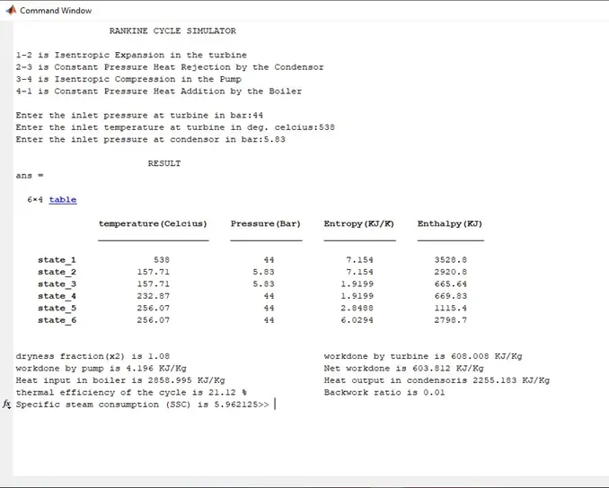
Plots:

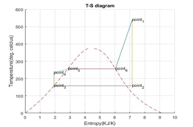
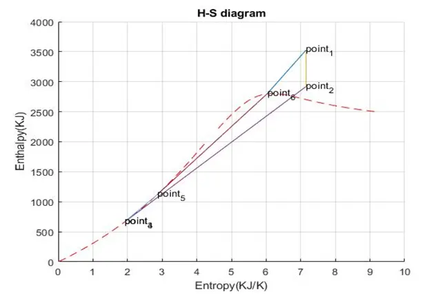
Reference: - http://www.thermopedia.com/content/1072

https://en.wikipedia.org/wiki/Rankine_cycle