Week 8 - Simulating Cyclone separator with Discrete Phase Modelling

Abstract:

A CFD analysis of a cyclone separator is performed. The separation efficiency is found out. Firstly the diameter of the particles is varied. Then the velocity at the inlet is varied with particles of constant diameter.The Physics of the problem is set up in Ansys Fluent. The Post -processing of the results obtained is done is CFD-Post.

Key-words- Cyclone separator, ANSYS,meshing, Ansys-Fluent, CFD-post ,separation efficiency, pressure drop

Introduction:

Cyclone separator or cyclones are devices that are used to remove particulate matter from flue gases using inertia method. This is one of the air pollution control devices called pre cleaners.Cyclone separators work much like acentrifuge but with a continuous feed of dirty air. In a cyclone separator, dirty flue gas is fed into a chamber. The inside of the chamber creates a spiral vortex, similar to a tornado. The lighter components of this gas have less inertia, so it is easier for them to be influenced by the vortex and travel up it. Contrarily, larger components of particulate matter have more inertia and are not as easily influenced by the vortex

Description of the project statement:

1. With varying the particle diameter, at a constant velocity at inlet the flow is simulated. separation efficiency is found out.

2. With varying the velocity at the inlet , at constant diamter of the particles, the flow is simulated. separation efficiency and pressure drop in the cases is found out.

Changing particle diameter from 1 micrometer to 5 micrometer , with velocity as 3 m/s:

• Geometry:

The cad file is imported into the spaceclaim. Fluid volume is extracted from the geometry by using the prepare option.

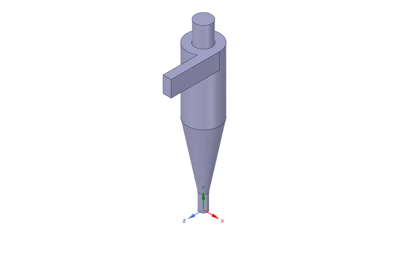
• Meshing:

Ansys mesher is openned. The default meshing that ansys does donot yield good results as there are only 4 cells in the inlet.

element size	0.006 meters
nodes	73004
number of elements	372662

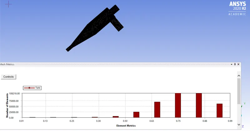
element quality:

minimum	4.2076e-002
maximum	1
average	0.83896
standard deviation	9.3504e-002

aspect ratio :

minimum	1.1583
maximum	46.586
average	1.8455
standard deviation	0.4698

skewness:

minimum	5.9871e-006
maximum	0.98689
average	0.22576
standard deviation	0.11675

orthogonal quality:

minimum	1.316e-002
maximum	0.99356
average	0.77249
standard deviation	0.11426

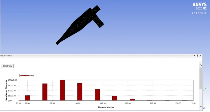
maximum corner angle :

minimum	70.576 degree
maximum	157.61 degree
average	96.21 degree
standard deviation	12.107 degree

The corresponding images are attched element quality, aspect ratio,skewness, orthogonal quality,maximum corner angle respectively:

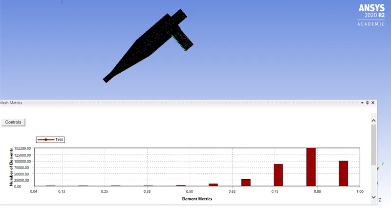
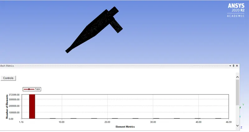
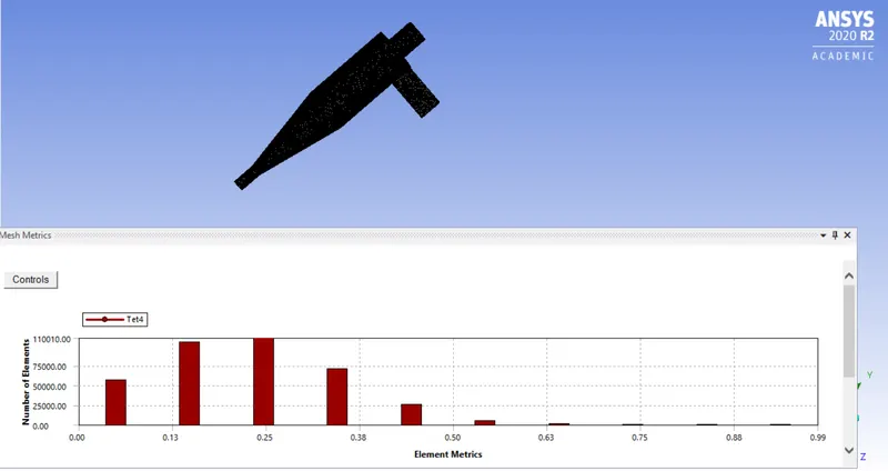
Providing named selection:

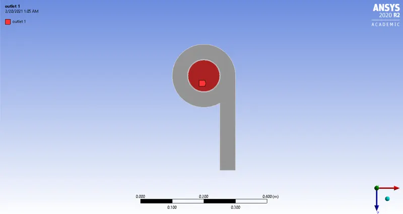
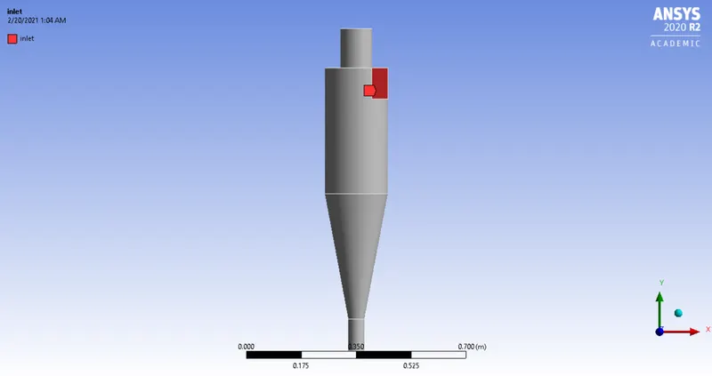
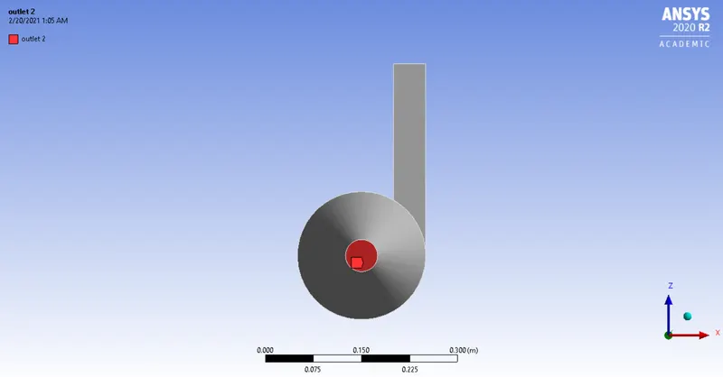
The face selecting tool is selected. The inlets , outlet (top) and outlet(bottom) is named. The inlet is through which the particles enter the lighter impurities escape through the top , and the heavier impurities are trapped in the bottom.

outlet(top),inlet and outlet(bottom) respectively are shown below

• Solving:

Physics set up:

1) Generall conditions:

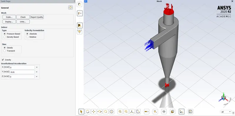
This analysis involves the orientation of the cyclone separator. As it is in the x-y plane, the accleration due to gravity needs to be turned on. As accelaration due to gravity acts upwards, the g value is assigned as -9.81 in the positive y axis.

Pressure based solver is used. Steady state analysis is done and the velocity formulation is normal to the boundary and absolute.

2) Physics set up:

• Turbulence modelling:

The K-epsilon(2 equation) model with RNG and swirl dominated flow is selected. The wall mofunctions are standard wall functions.

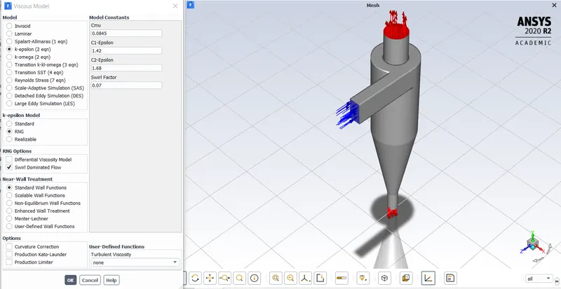
Since temperature is not involved, the Energy is not turned on.

• DPM:

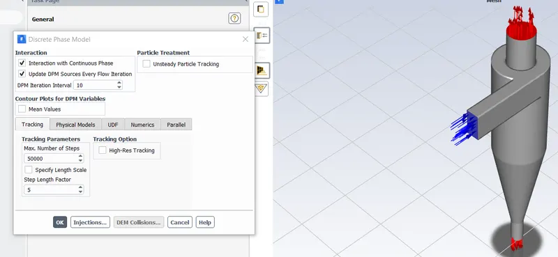
Discrete phase modeling is opted for.

The model is enabled for interaction with the continuous phase. DPM interval level is 10.

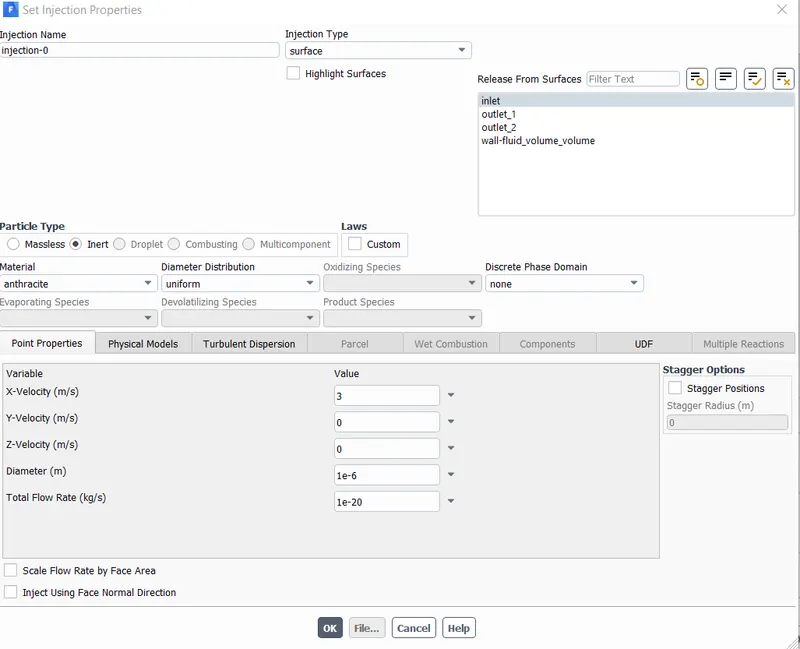
For injection, the particle type is inert. From fluent database , anthracite is selected. It is released from the inlet, with velocity in the x-direction being 3m/s. This velocity may be manipulated further. The particle diameter chosen for the first analysis is one micrometers. The particle diameter is varied from one micrometer to five micrometers to calculate the separation efficiencies.

• Boundary conditions:

The boundary conditions are provided to three named selections, inlet , outlet(1)top and outlet(2) bottom.

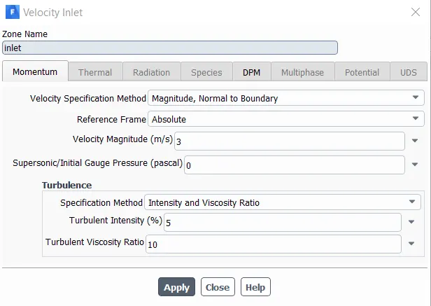
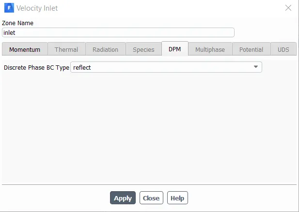
For inlet, the momentum conditions are v3locity is 3m/s in the x direction , being absolute and normal to the boundary. The DPM condition is reflect. This signifies that the particles are not allowed to escape or get trapped in the inlet.

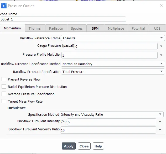
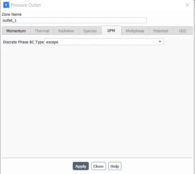
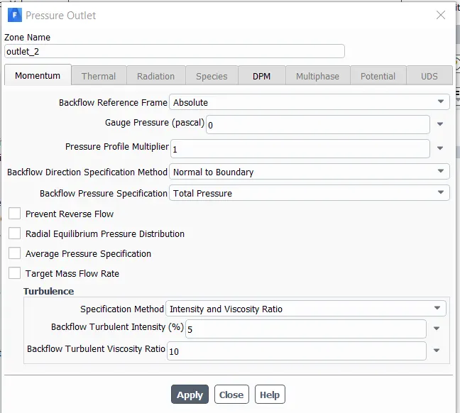
For the top outlet, the Momentum condition is vasically pressure condition, The DPM condition is escape. Particles can escape from this Boundary

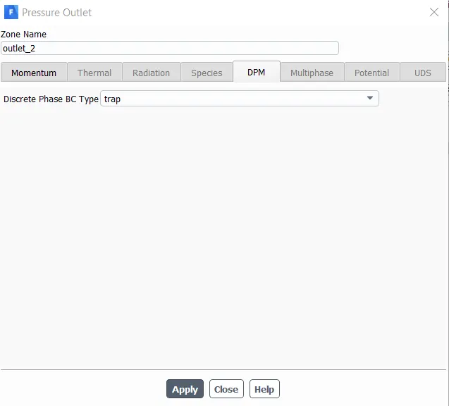
The bottom outlet is also a pressure outlet, with the DPM condition being trap.

• Solution methods:

The pressure velocity coupling is chosen as COUPLED scheme. The gradient being least square cells based. Pressure,Momentum, Turbukent kinetic energy and turbulent dissipation rate is second order upwind.

• Initialization:

Standard initialization is done with flow from inlets.

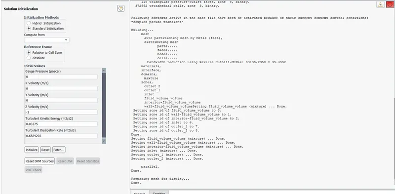
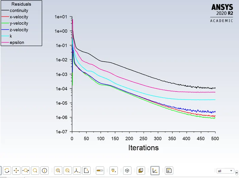
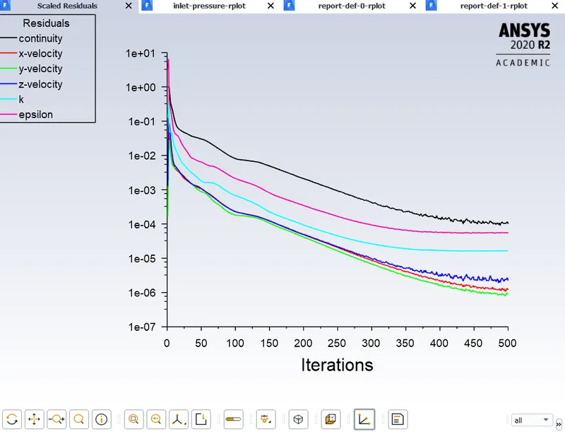
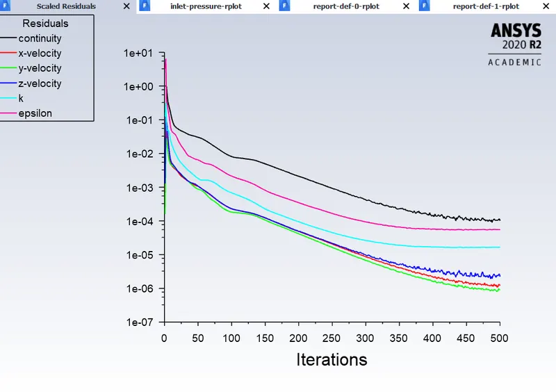
The analysis is done for 500 iterations.

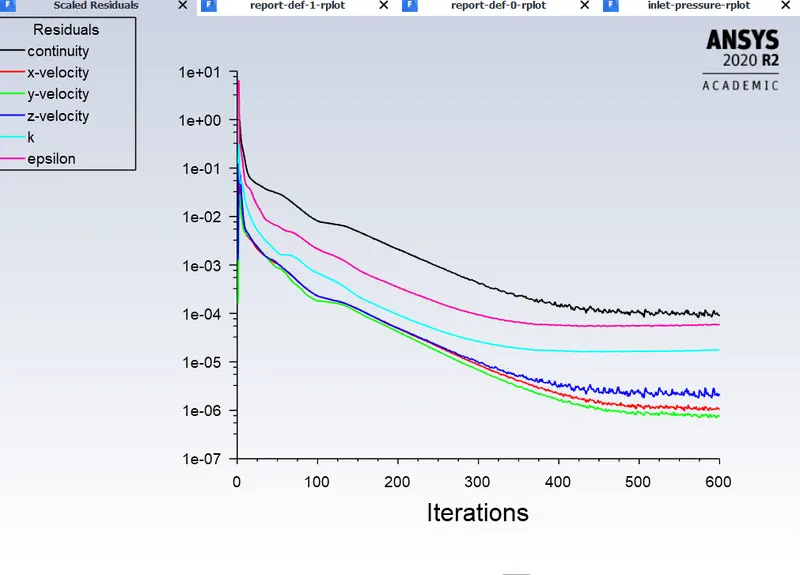
The scaled residuals plot :

• Post processing:

The data is exported from the fluent to CFD post to visualize the results. Opening CFD post , the particle histry data is imported.

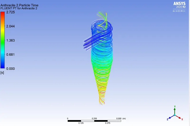
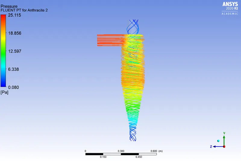
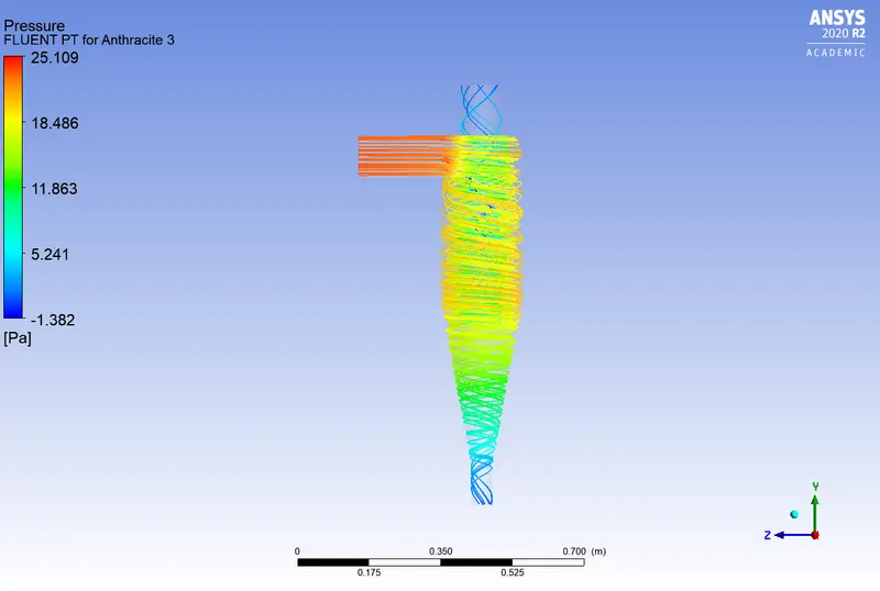
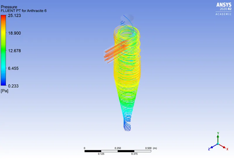
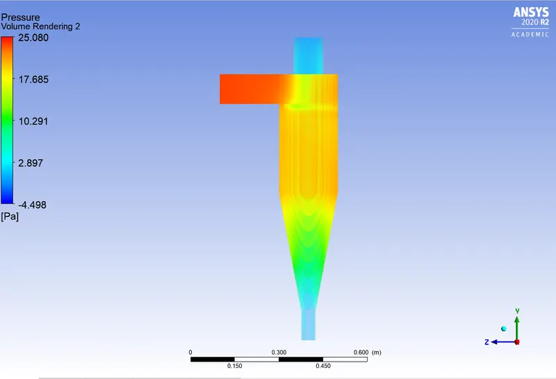
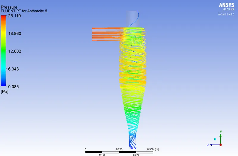
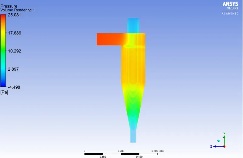
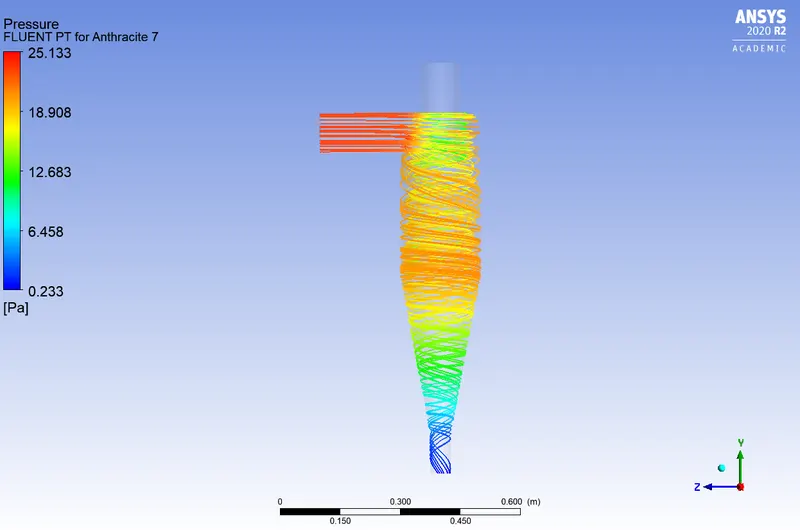
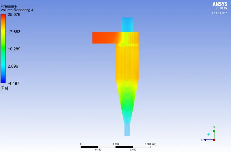
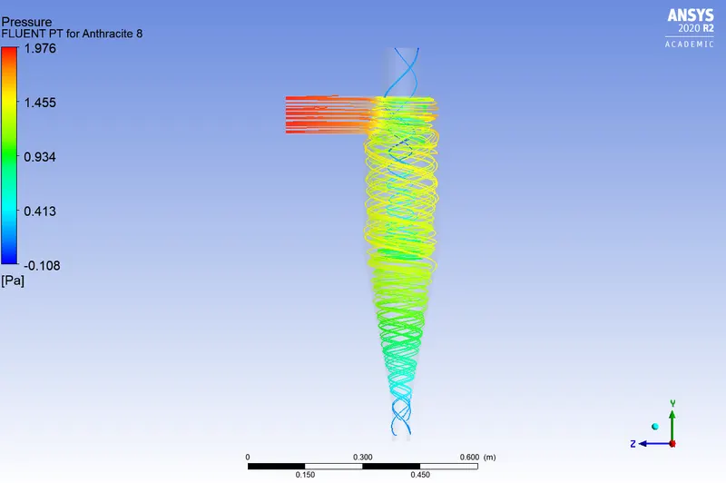
From the pressure plot, it can be inferred that the pressure is much higher at the inlets where as lowes at the both outlets.

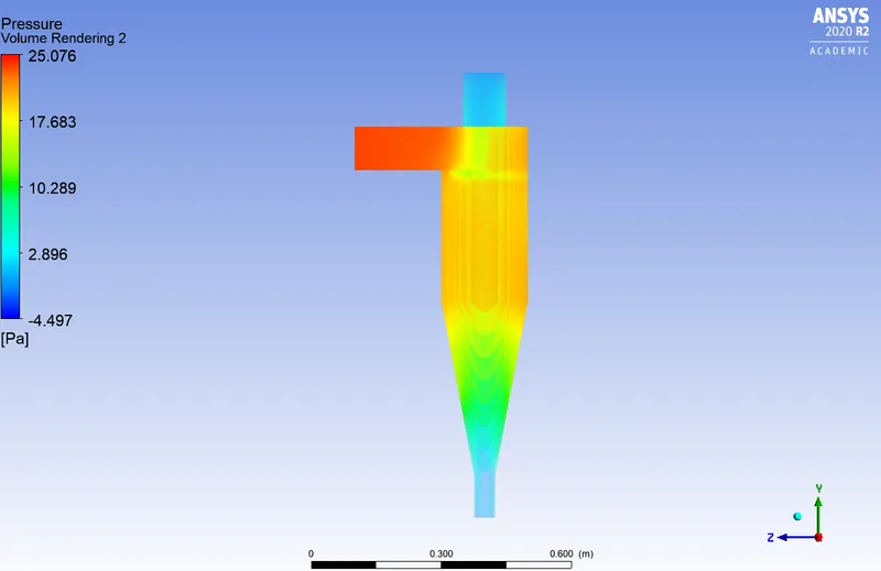
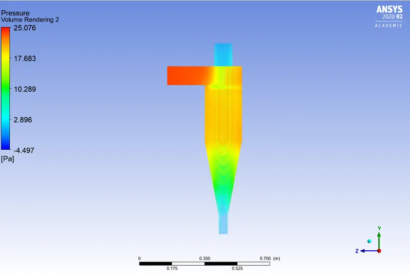
The volume can be rendered with pressure as the parameter,

tracked	escaped	trapped	incomplete
288	74	54	160

Separation efficiency:

(number of particles trapped/number of particles tracked )*100

So, separation efficiency = (54/288)*100 = 18.75%

Diameter of the particles = 2 micrometers

The set up of the physics is same as the above case , except the particle diameter in the DPM modelling is increased to 2 micrometers. All other boundary conditions, initialisation and the solution methods are same.

Scaled residuals :

Tracked	escaped	trapped	incomplete
288	57	191	40

Separation efficiency = (191/288)*100=66.31%

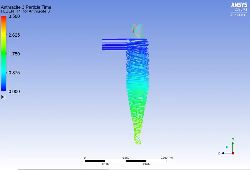
• Post-process visuals:

The volume rendered with pressure as variable is:

Diameter of the particles = 3 micrometers:

The DPM interval is set to 5 iterations

Tracked	Escaped	Trapped	Incomplete
288	35	192	61

Separation efficiency= (192/288)*100 = 66.66%

The scaled residuals are:

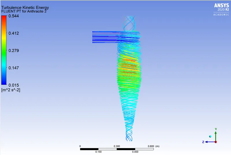
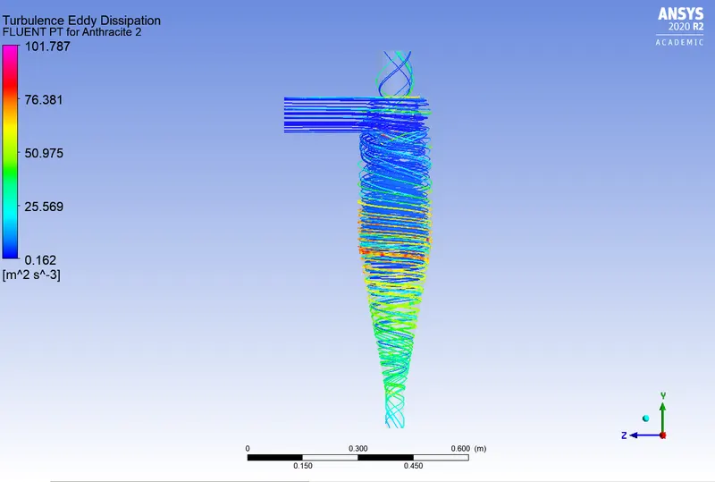
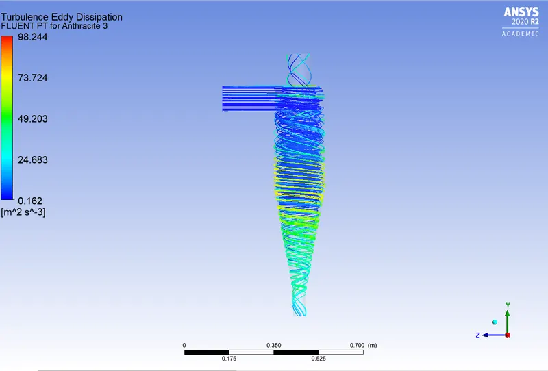
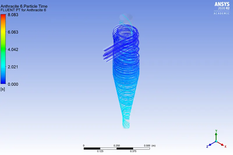
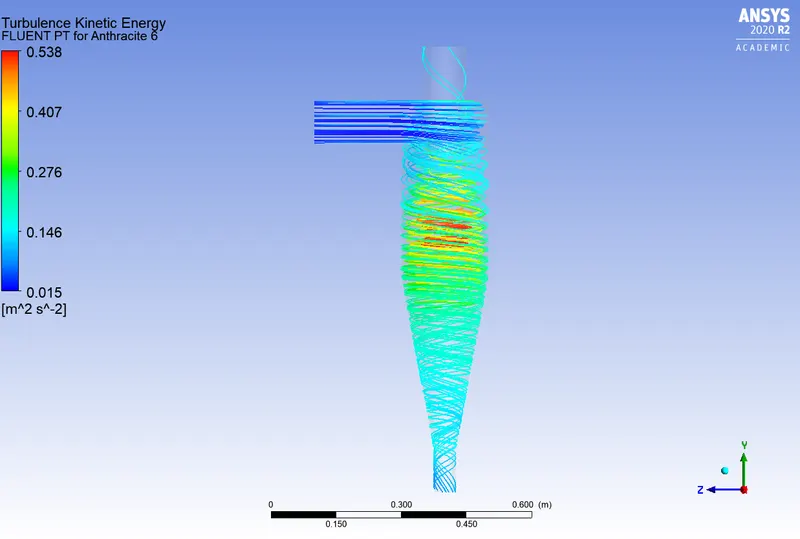
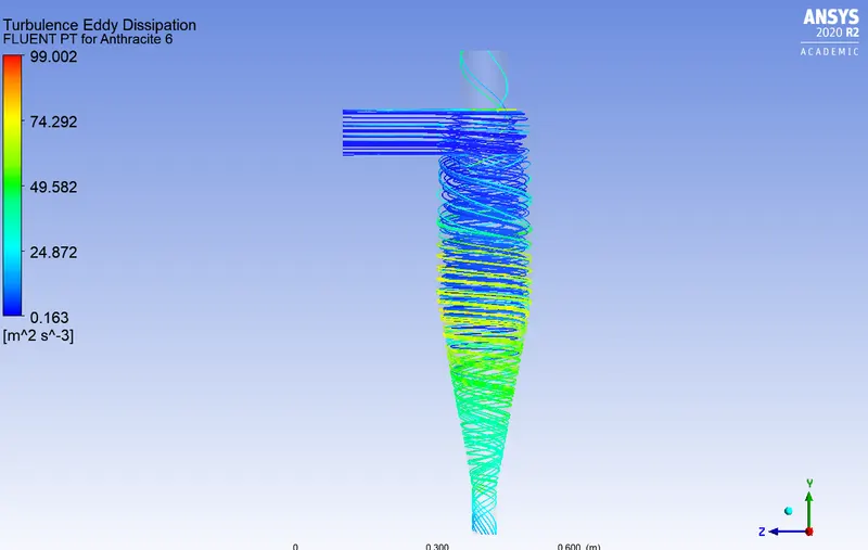
The Post proccesiing plots of pressure, turbulent kinetic energy, turbulent eddy dissipation , volume rendering with pressure variable are:

Diameter of the particles = 4 micrometers:

To decrease the number of particles incomplete , the DPM interval level is reduced. it is made 5.

All other parameters are same.

Tracked	Escaped	Trapped	Incomplete
288	7	219	62

Separation efficiency = (219/288)*100 = 76.04%

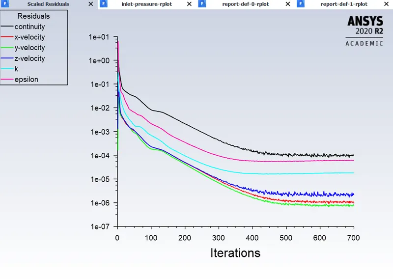
Scaled residuals:

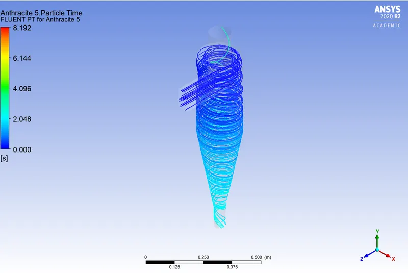
The post processing data are:

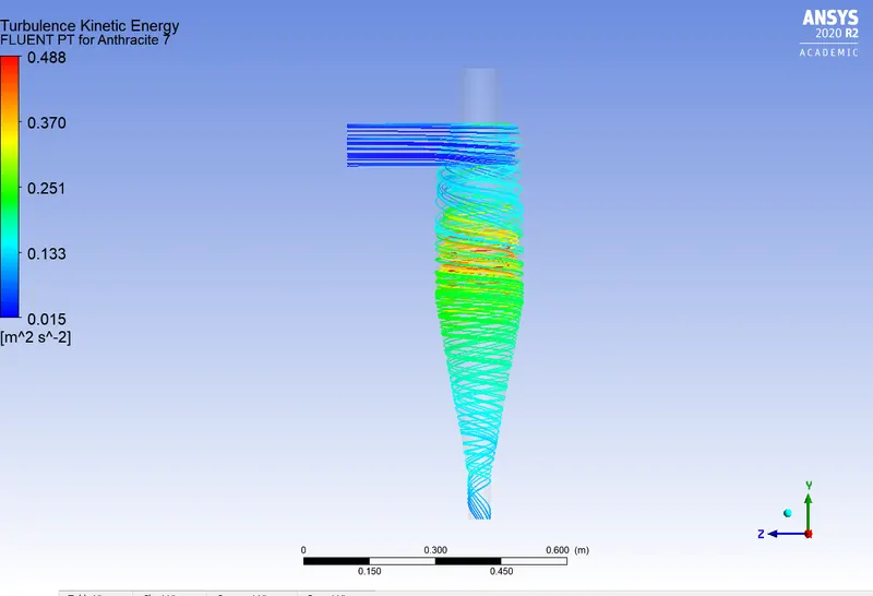
The turbulent kinetic energy and the turbulent eddy dissipation distribution is shown below.

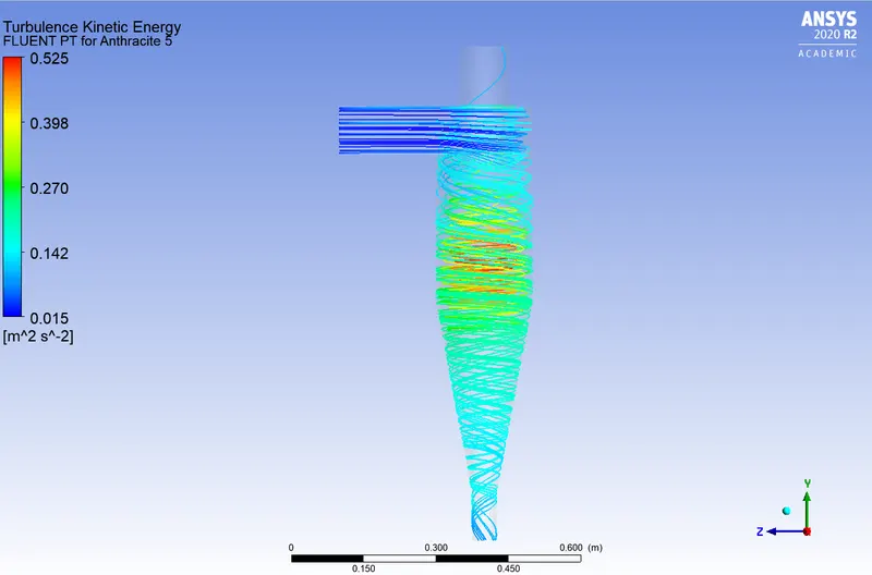
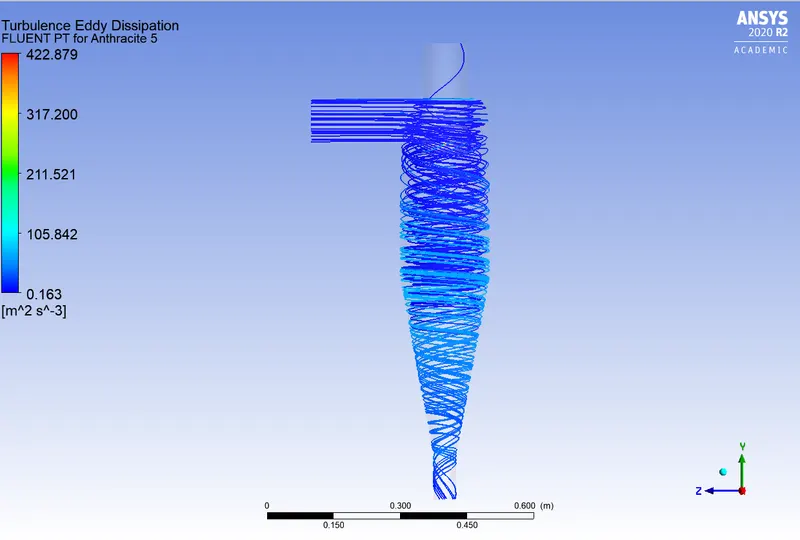
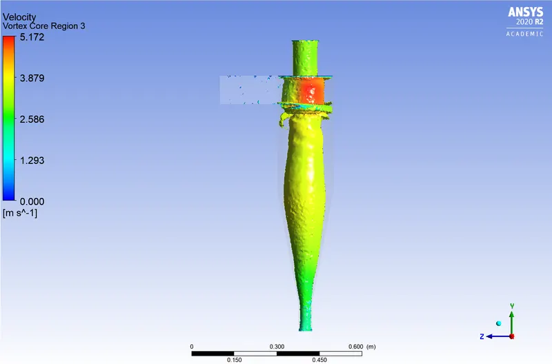
The volume rendered with pressure as variable and the velocity vortex is shown below

Diameter of particles = 5 micrometers:

The DPM interval is set to 2 iterations.

All other conditions are same.

Tracked	Escaped	Trapped	Incomplete
288	0	267	21

Separation efficiency = (267/288)*100 = 92.70%

The scaled residuals are:

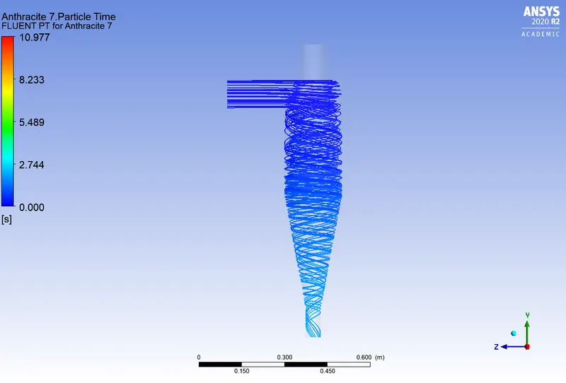
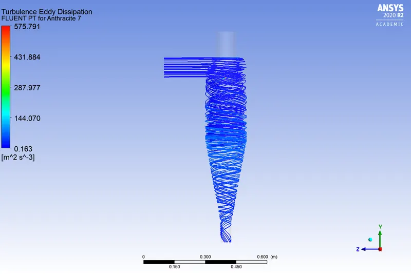
The post -processed visuals of pressure, turbulent kinetic energy, turbulent eddy dissipation , volume rendering with pressure as variable are as follows:

Vortex core region with different swirl strength :

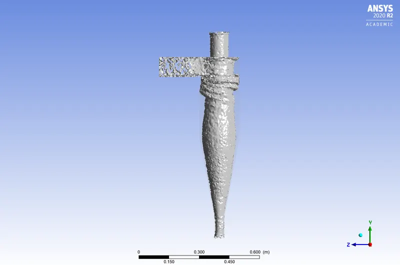swirl strength = 0.012

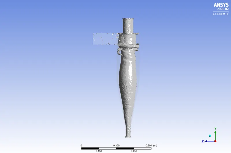swirl strength = 0.055

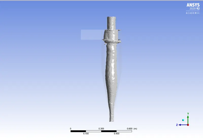swirl stength = 0.12

• Final efficiency tabulation:

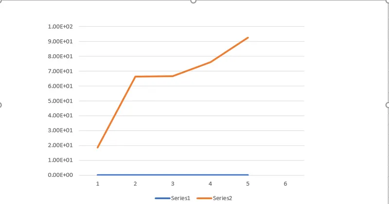
Particle diameter	Velocity	Efficiency(%)
1e-6	3	18.75
2e-6	3	66.31
3e-6	3	66.60
4e-6	3	76.04
5e-6	3	92.70

Plot of efficiency of the cyclone separator vs the diameter of the particles

The separation efficiency is plotted along the Y axis and the particle diameters along the X axis. This is done in Microsoft Excel

• Validation of results obtained by CFD analysis from the Analytical methods:

The various analytical models to calculate the separation efficiency of cyclone separators are:

1) Iozia and Leith model:

Developed from the basis of force balance. The model assu,es that the particle carried by the vortex endures the influence of two forces : A centrifugal force Z and a flow resistence W. The separation efficiency can be written as :

`eta(i)=(1/((1+(d(pc))/(d(p)))^beta)))`

`beta = 0.62-0.87*(ln(d(pc))/100)+5.21*ln((a*b)/D^2)+1.05(ln((ab)/D^2)^2)`

d(pc)= 50% cut size

`d(pc)=((9*mu*Q)/(pi*rho(p)*Z(c)*v^2))^0.5`

Z(c) = core length and d(c) = core diameter.

Here d(c)<B;

so, Z(c) = H-S

In our model :

All dimensions are in meters.

D(e)=0.1

D=0.2

b=0.05

a=0.1

h=0.4

H=0.8

B=0.05

Rho=1550 kg/m^3

mass flow rate = 1e-20

Calculating Q = mass flow rate * Rho

And putting the values in the equation of efficiency, we get , separation efficiency = 98%

error = (98-92.70)/98 *100 =5.40 %

The efficiency can be increased by incresing the number of cells in the mesh.

2)Koch and Licht model:

Koch and Licht inherently described the turbulent nature of cyclones and distribution of gas residence times within the cyclone. They attributed by the two following assumptions:

• The tangential velocity of the particle is equal to the tangential velocity of the gas flow. There is no slip in the tangential direction between gas nad particle.
• The tangential velocity is related to the radius of the cyclone by uR^n = constant

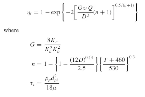This is the formula for the grade efficiency

3) Li and Wang model:

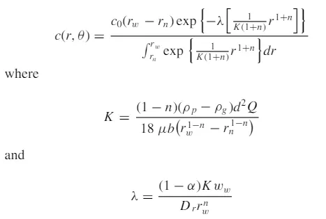
The Li and Wang model includes the particle bounce or rentrainment or turbulent diffusion at the cyclone wall.A two dimensional analytical expression for the particle distribution is obtained. The Li and Wang model is based on the following assumptions:

• The radial particle velocity and the radial concentration profile are not constant for the uncollected particles within the cyclones.
• Boundary conditions with the consideration of turbulent diffusion coefficient and particle bounce reentrainment on the cyclone wall are

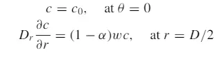
• The tangential velocity is related to the cyclone radius by uR^n=constant

The concentration distribution is given as :

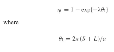
The expression for collection efficiency for particles of any size is given as:

• manipulation of the inlet velocity from 1m/s to 5m/s for a fixed particle diameter :

Case 1 = velocity = 1m/s

particle diameter = 5e-6 meters

The set up of the problem is same as above.

Tracked	Trapped	Escaped	Incomplete	pressure drop
288	12	27	249	2.084 (pa)

Separation efficiency = (12/288)*100 = 4.166%

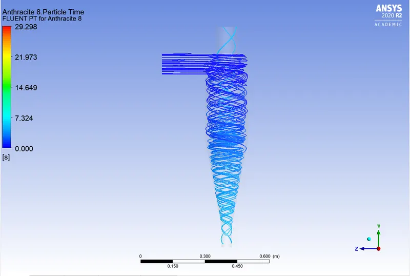
The post processed plots are:

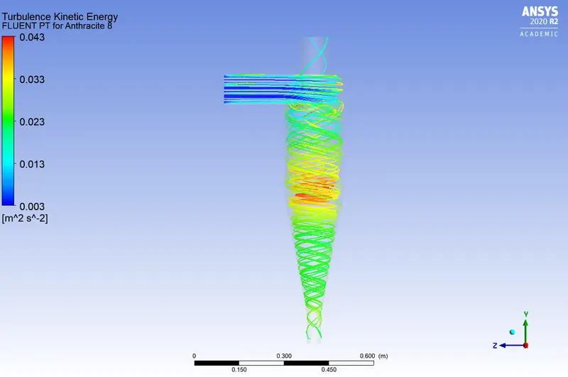
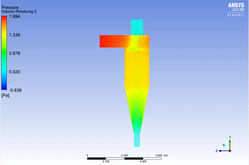
Case 2= velocity = 5m/s:

Tracked	Trapped	Escaped	Incomplete	Pressure drop
288	288	0	0	70.828(Pa)

Separation efficiency = (288/288)*100 = 100%

The scaled residuals are:

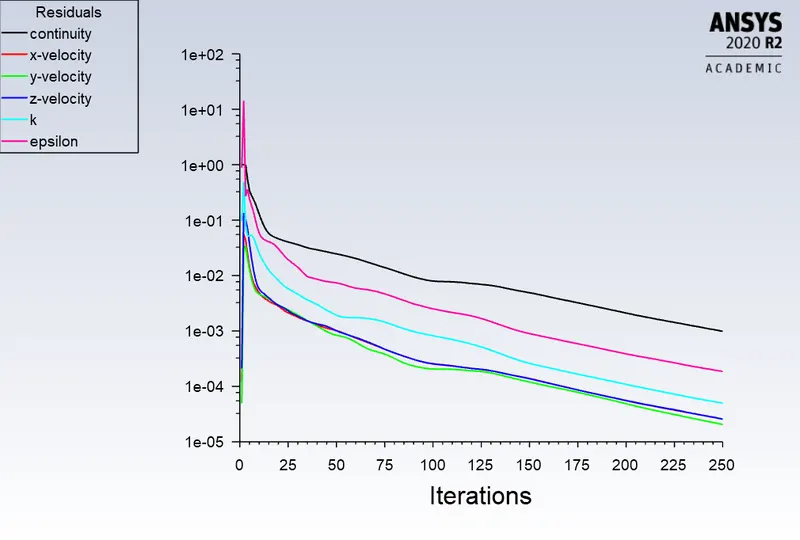
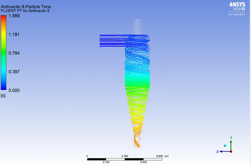
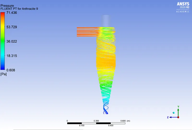
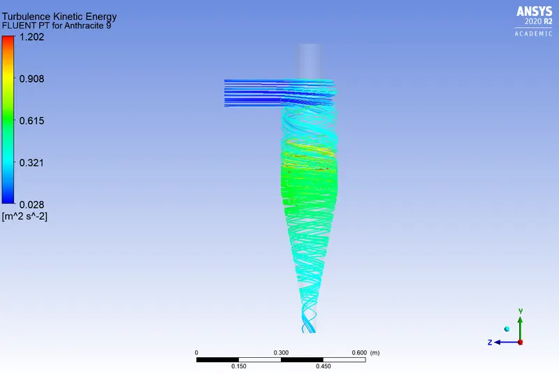
The time for which the particles remain inside the cyclone separator , The pressure distribution and the turbulent kinetic energy distributin are:

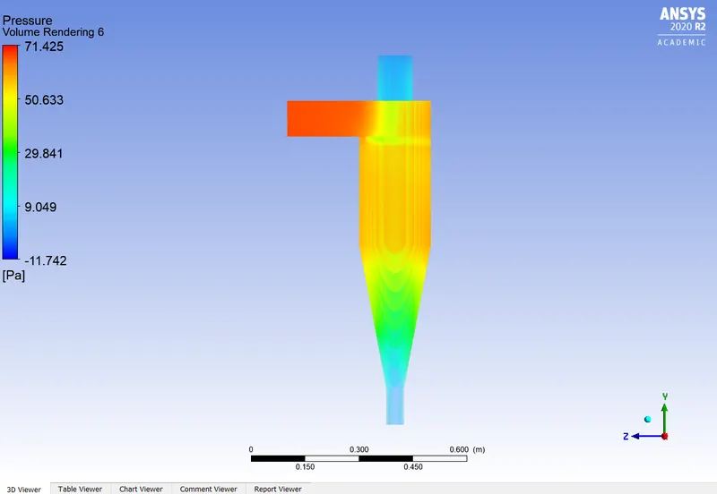
The volume rendered with pressure as variable is:

Compiling the results:

Velocity of flow	Particle diameter	Separation efficiency	Pressure drop
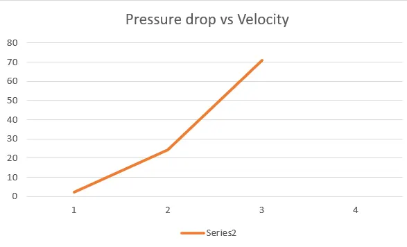
1(m/s)	5e-6	4.166%	2.084(Pa)
3(m/s)	5e-6	92.70	24.36(Pa)
5(m/s)	5e-6	100%	70.828(Pa)

If the prssure drop and the Velocity of flow is plotted against each other:

• Conclusion:

A complete simulation of cyclone separator is performed. The quality of the results obtained can be improved by using more number of elements in the analysis , which couldnt be done here due to an academic license and less computational power.

The Validation of the model from the literature available shows , a good amount of confidence is reached with the analysis.