Week 8 - Simulating Cyclone separator with Discrete Phase Modelling

Simulating Cyclone separator with Discrete Phase Modelling

Aim: To perform analysis on cyclone separator and calculate the separation efficiency and pressure drop.

Objective:

1. To write a few words about any four empirical models used to calculate the cyclone separator efficiency.
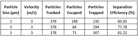
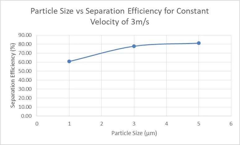
2. To perform an analysis on a given cyclone separator model by varying the particle diameter from 1 μm to 5 μm and calculate the separation efficiency in each case. Discuss the results. [Use both the velocity's as 3m/sec.]
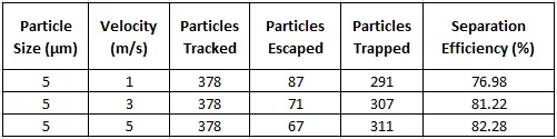
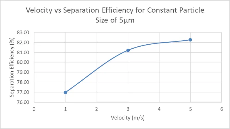
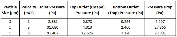
3. To perform an analysis on a given cyclone separator model by varying the particle velocity from 1 m/sec to 5 m/sec and calculate the separation efficiency and pressure drop in each case. Discuss the results. [Use particle diameter size as 5 μm for all cases & keep flow velocity same as particle velocity]

Boundary Conditions:-

Inlet and wall:- Reflect

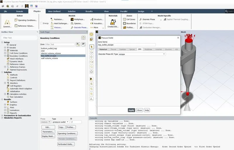
Outlet(Top):- Escape

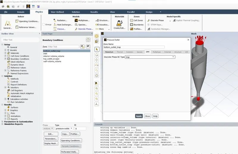
Outlet(Bottom/dustbin) - Trap

CYCLONE SEPARATOR

A cyclone separator is an economical device for removing particulate solids from a fluid system. The induced centrifugal force is tangentially imparted on the wall of the cyclone cylinder. This force, with the density difference between the fluid and solid, increases the relative settling velocity.

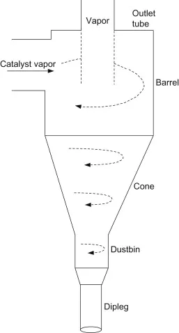
Cyclone separators are extremely important toward the successful operation of the cat cracker. Their performance impacts several FCC performance factors, including the additional cost of fresh catalyst makeup, extra turnaround maintenance costs, the allowable limits on emission of particulates, and the incremental energy recovery in the WGC, and hot gas expander.

Designing an “optimum” set of cyclones requires a balance between the desired collection efficiency, pressure drop, space limitations, and installation cost. The cyclone process and mechanical design recommendations are shown in table below

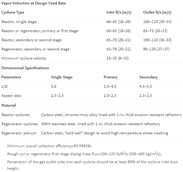
Cyclones are devices that employ a centrifugal force generated by a spinning gas stream to separate particles from the carrier gas. Their simple design, low maintenance costs, and adaptability to a wide range of operating conditions such as sizes and flow rates make cyclones one of the most widely used particle removal devices. By using suitable materials and methods of construction, cyclones may be adapted for use in extreme operating conditions: high temperature, high pressure, and corrosive gases. Cyclones are important particle removal devices in both engineering and process operations.

CYCLONE DESIGN

The reverse flow cyclones with tangential inlet, Figure 1, are most often used for industrial gas cleaning. The dimensions of the cyclones used in this study are given in Table 1. The inflowing fluid rotates within the main body of the chamber and is constrained to follow a spiral flow path. Any particles suspended within the fluid are subjected to an enhanced radial acceleration. The larger particles migrate outwards to the cone wall where they travel in a downward spiral to the base of the chamber and exit at the underflow. The smaller particles migrate more slowly and therefore their distribution across the flow changes little. Those in the centre are captured in the upward flow and spiral upward and out through the vortex finder. The remainder is discharged with the coarse fraction at the underflow.

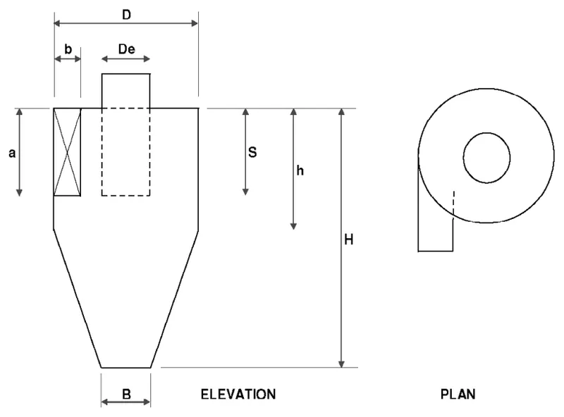
Figure 1 : Tangential cyclone configuration

Table 1 :

CYCLONE EFFICIENCY EMPIRICAL MODELS

IOZIA AND LEITH MODEL

Iozia and Leith (1990) logistic model is a modified version of Barth (1956) model which is developed based on force balance. The model assumes that a particle carried by the vortex endures the influence of two forces: a centrifugal force, Z, and a flow resistance, W. Core length, z_c , and core diameter, d_c , are given as

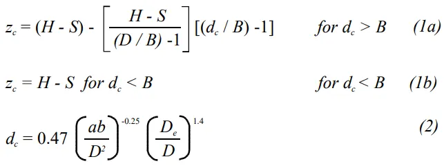
The addition made by Iozia and Leith on the original Barth (1956) model are the core length z_c and slope parameter β expression which is derived based on the statistical analysis of experimental data of cyclone with D = 0.25 m. The collection efficiency η_i of particle diameter d_pi can be calculated from

where d_pc is the 50% cut size given by Barth (1956)

LI AND WANG MODEL

The Li and Wang (1989) model includes particle bounce or re-entrainment and turbulent diffusion at the cyclone wall. A two-dimensional analytical expression of particle distribution in the cyclone is obtained. Li and Wang model was developed based on the following assumptions:

The radial particle velocity and the radial concentration profile are not constant, for uncollected particles within the cyclones.

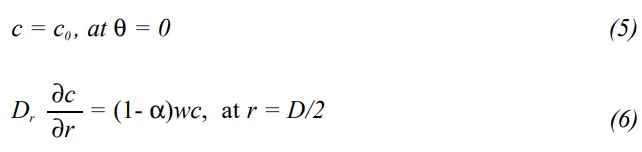
Boundary conditions with the consideration of turbulent diffusion coefficient and particle bounce re-entrainment on the cyclone wall are:

The tangential velocity is related to the radius of cyclone by:

uRⁿ = constant.

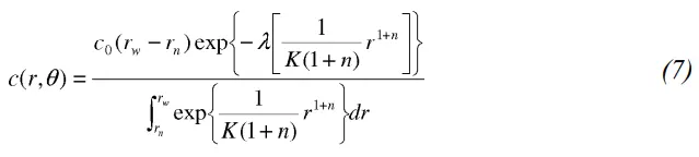
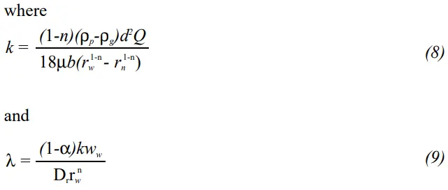
The concentration distribution in a cyclone is given as:

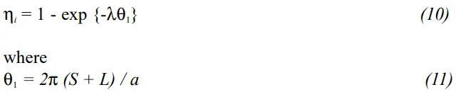
The resultant expression of the collection efficiency for particle of my size is given as

KOCH AND LICHT MODEL

Koch and Licht (1977) collection theory recognized the inherently turbulent nature of cyclones and the distribution of gas residence times within the cyclone. Koch and Licht describe particle motion in the entry and collection regions with the additional following assumptions:

The tangential velocity of a particle is equal to the tangential velocity of the gas flow, i.e. there is no slip in the tangential direction between the particle and the gas.

The tangential velocity is related to the radius of cyclone by: uRⁿ = constant. A force balance and an equation on the particles collection yields the grade efficiency η_i .

where

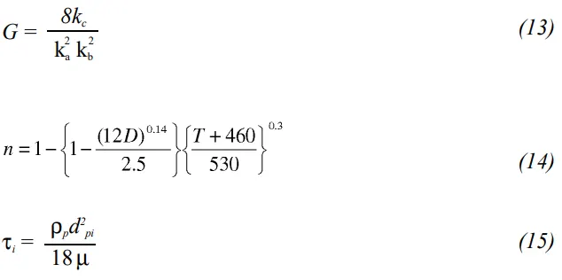
G is a factor related to the configuration of the cyclone, n is related to the vortex and τ is the relaxation term.

LAPPLE MODEL

Lapple (1951) model was developed based on force balance without considering the flow resistance. Lapple assumed that a particle entering the cyclone is evenly distributed across the inlet opening. The particle that travels from inlet half width to the wall in the cyclone is collected with 50% efficiency. The semi empirical relationship developed by Lapple (1951) to calculate a 50% cut diameter, d_pc, is

where N_e is the number of revolutions

The efficiency of collection of any size of particle is given by

DICRETE PHASE MODEL

The discrete Phase Model is a subsection of Multiphase flows. A discrete phase model (DPM) is used when the aim is to investigate the behavior of the particles from a Lagrangian view and a discrete perspective. The difference between the Lagrangian and the Eulerian view is that fluid behavior in the Lagrangian view is examined based on particle tracking of a particulate flow, whereas fluid behavior is considered in the Eulerian view based on the assumption of a finite volume element in the fluid flow path.

In Discrete Phase Model, the continuous phase is solved using Navier-Stokes equations. At the same time, the discrete phase is simulated by tracking a large number of particles, bubbles, or droplets passing through the calculated continuous flow field. It should be noted that the discrete phase can exchange momentum, mass, and energy with the continuous phase. This method can be made much simpler by ignoring the interaction of particles (as well as droplets and bubbles) with each other. Of course, this can happen when the discrete phase, even with a large mass, has a much smaller volume (less than 10%) than the continuous phase. After each iteration of the continuous phase calculations, the particle paths are calculated and determined separately.

Dense Discrete Phase Model (DDPM)

The dense discrete phase model (DDPM) is a Lagrangian parcel-based approach that models particle collisions and uncorrelated translations using the kinetic theory of granular flows (KTGF). This approach has numerous advantages over the established Eulerian two-fluid model (TFM). These include better resolution of particle clusters and bubbles, more natural incorporation of particle size distributions and better handling of crossing particle jets/clusters. In this study, results from the DDPM are compared to dedicated experiments and TFM simulations over a wide range of fluidization velocities, particle sizes, and bed loadings. Special attention was given to ensure that the frictional effects typical of such dense particle flows are accounted for. The DDPM proved capable of reproducing the good fit to experiments achieved by the TFM on a significantly coarser mesh.

Discrete Element Method (DEM)

The discrete element method (DEM) is an intuitive method in which discrete particles collide and other surfaces during an explicit dynamic simulation. Typically, each DEM particle represents a separate grain, tablet, shot peen, etc. DEM does not apply to situations in which individual particles undergo complex deformation. Therefore, DEM is, unlike conceptually, more straightforward than the smoothed particle hydrodynamic (SPH) method in which groups of particles collectively model a continuum body. For example, DEM is well-suited for particle mixing applications. In this application, DEM is used to model the initially separated blue and white particles, and rigid finite elements are used to model two mixing augers and the box-shaped container. Another example of using DEM for a mixing application is described in the Mixing of granular media in a drum mixer.

Discrete Phase Simulations in ANSYS Fluent Software

Newton’s second law of motion explains the basic theory behind the discrete phase modeling process. As was mentioned in the previous paragraph, the continuous phase equations are solved first to obtain the flow field and its related parameters. Then, based on different projects, one may assume various forces that apply to the particulate phase. Finally, we can track each particle inside our continuous phase by coupling the Navier-Stokes equations with Newton’s equation.

The Discrete Phase in ANSYS FLUENT can be used to model different types of phenomena, including:

• calculation of the discrete phase trajectory using a Lagrangian formulation that includes the discrete phase inertia, hydrodynamic drag, and the force of gravity for both steady and unsteady flows
• prediction of the effects of turbulence on the dispersion of particles due to turbulent eddies present in the continuous phase
• heating/cooling of the discrete phase
• vaporization and boiling of liquid droplets
• combusting particles, including volatile evolution and char combustion to simulate coal combustion
• droplet breakup and coalescence
• Erosion or accretion

Various types of built-in forces can be applied to make the created project even more realistic, such as Thermophoretic, Brownian, Saffman forces, etc. Also, user-defined functions are always there for modeling the forces that are not predefined in the software.

These modeling capabilities allow ANSYS FLUENT to simulate a wide range of discrete phase problems, including particle separation and classification, spray drying, aerosol dispersion, bubble stirring of liquids, liquid fuel combustion, and coal combustion.

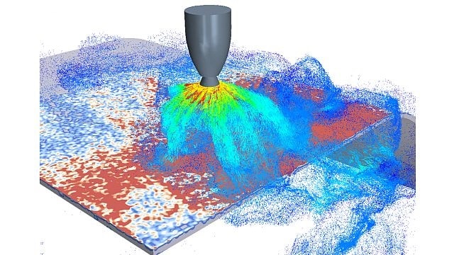
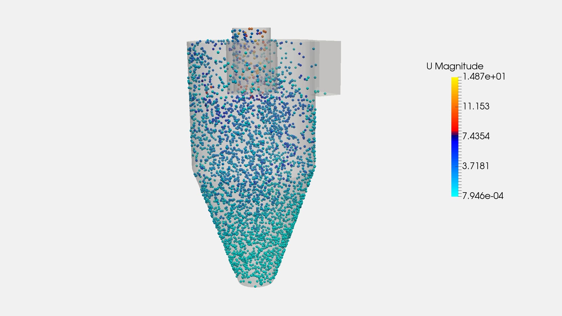
Simulation Cases Performed Using Ansys Fluent

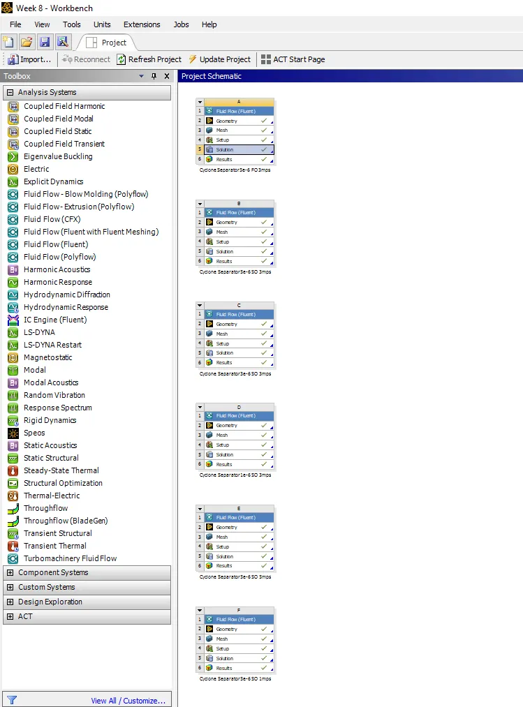
STEPS USED FOR SIMULATIONS

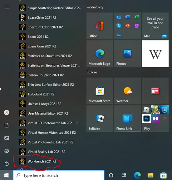
Click on red encircled "Workbench 2021 R2" as shown in the above image to start the simulation.

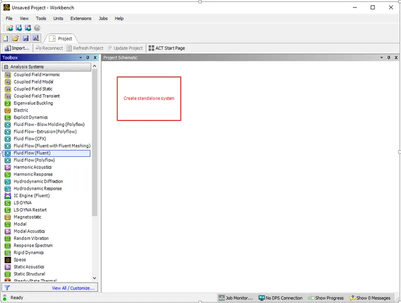
Click On Fluid Flow (Fluent) under Analysis Systems and drag it to create a standalone system. Rename the project as Cyclone Separator.

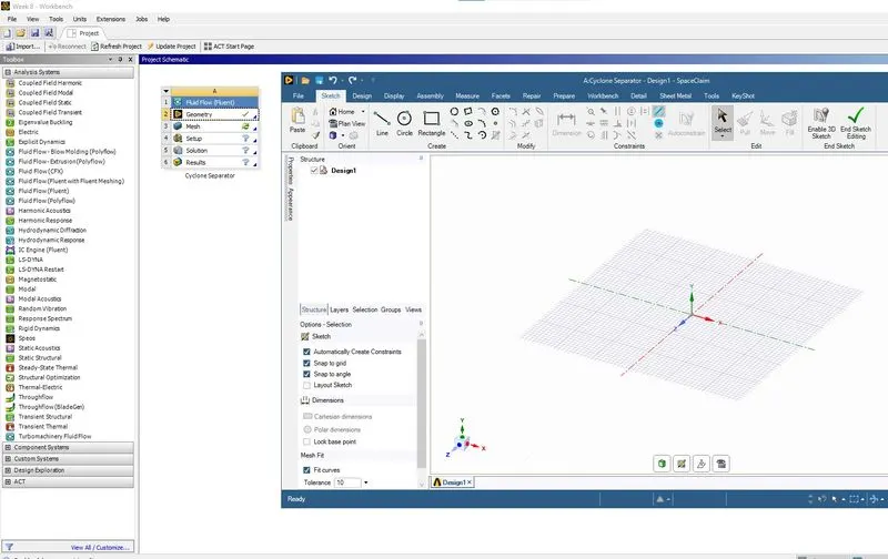
Click on the Geometry to open the space claim window.

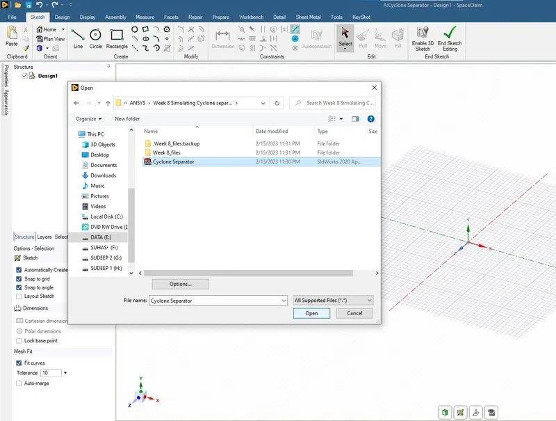
Open the Cyclone Separator.STEP file as shown in the above image.

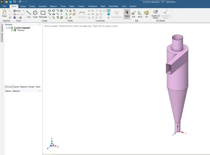
The preview of the cyclone separator as shown in the above image.

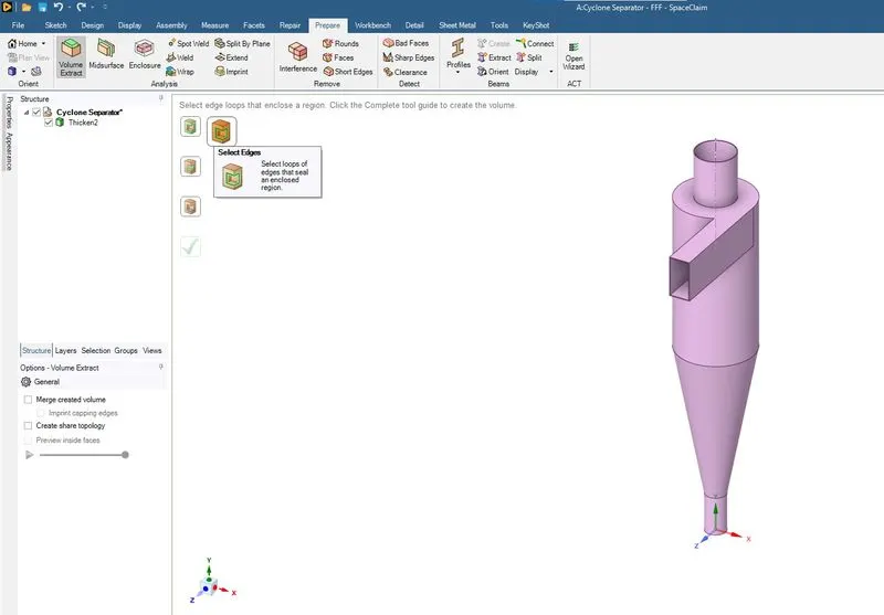
Volume Extract under the Prepare Tab is used to extract the fluid volume. Select edges is clicked to extract the fluid volume enclosed in the selected edges.

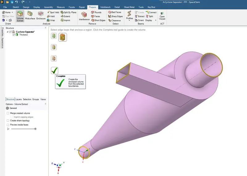
The edges are selected as shown in the above image and the green tick complete is clicked as shown in the abovw image.

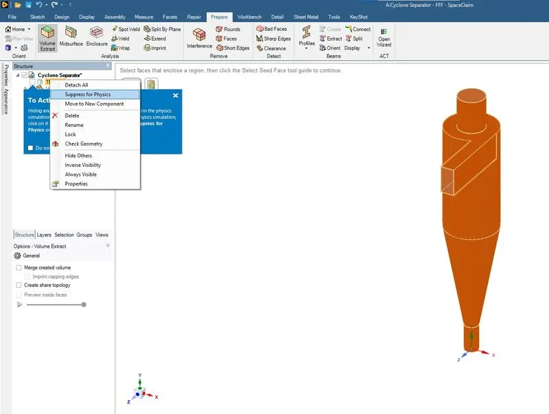
The sheet metal part is suppressed for physics as shown in the above image.

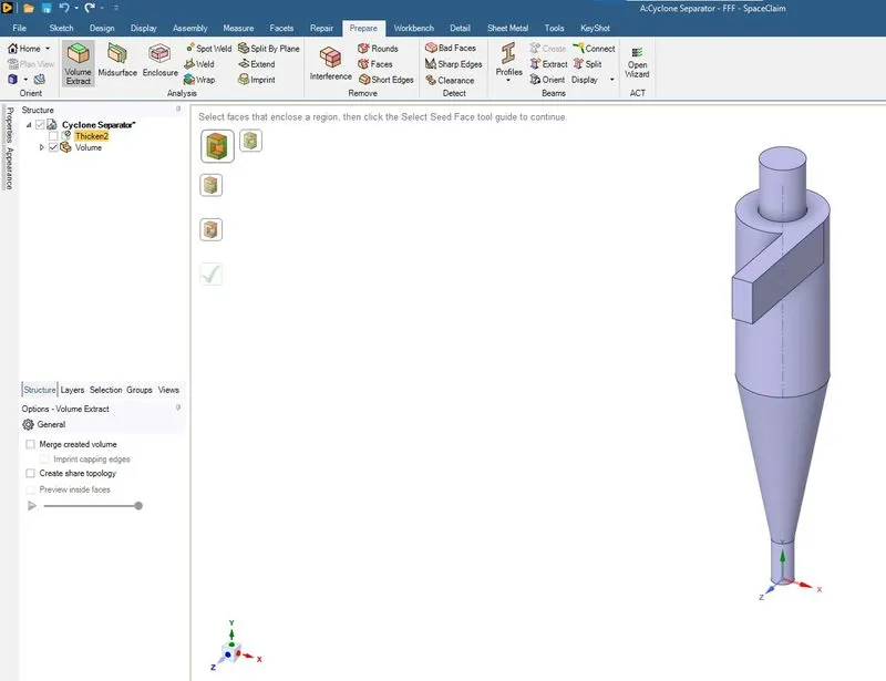
The preview of the extracted fluid volume as shown in the above image.

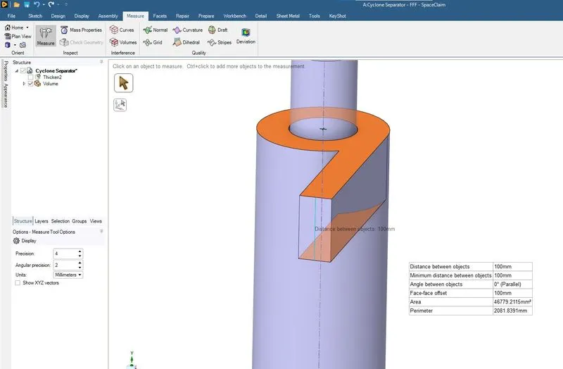
Measurement of the highlighted parameters

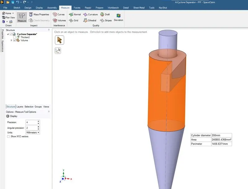
Maesurement of the highlighted parameters.

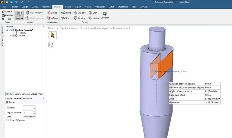
Measurement of the highlighted parameters.

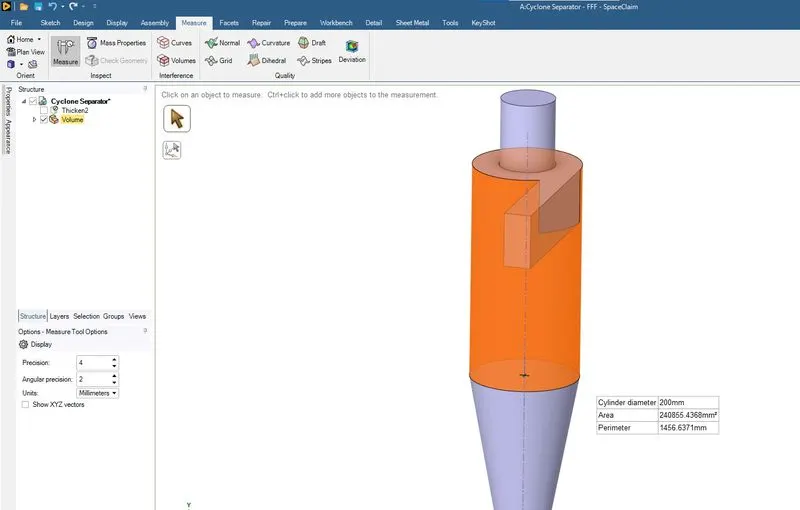
Measurement of the highlighted parameters.

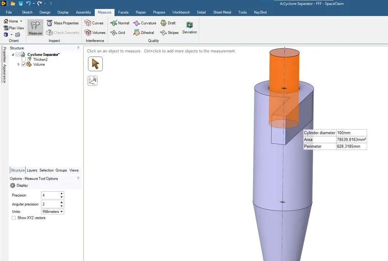
Measurement of the highlighted parameters.

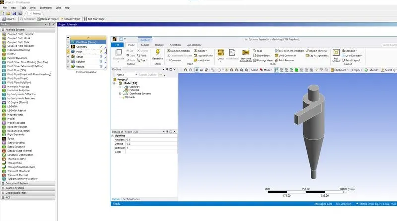
By clicking the Mesh option as shown in the above image, the meshing window is opened.

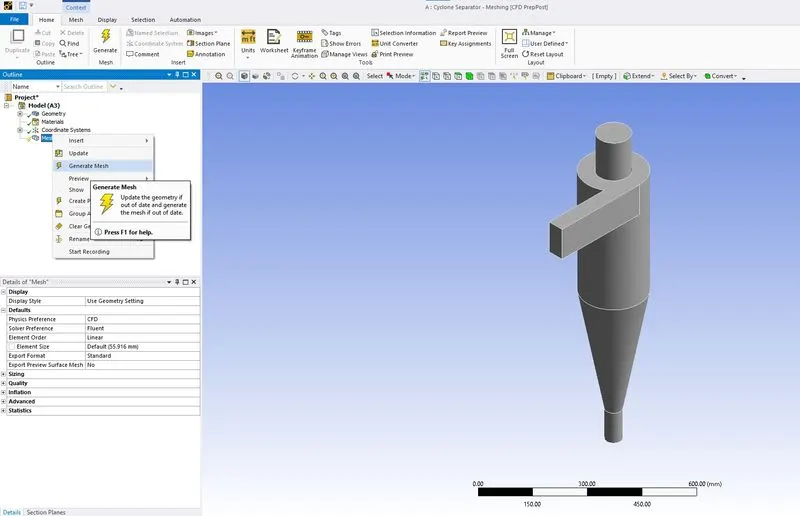
By clicking the generate mesh as shown in the above image, a default mesh is generated.

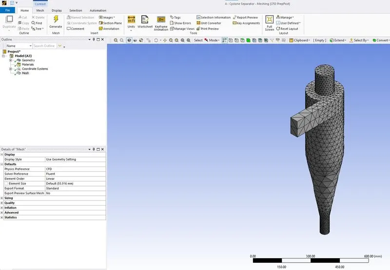
The preview of the default mesh generated.

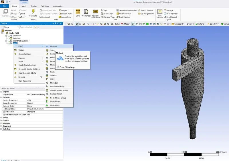
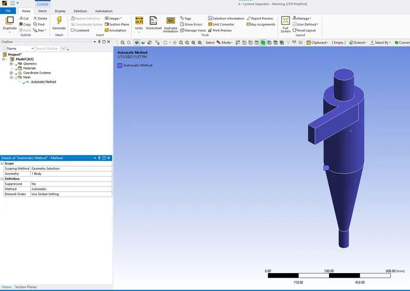
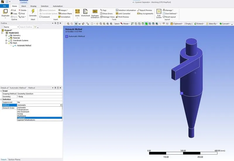
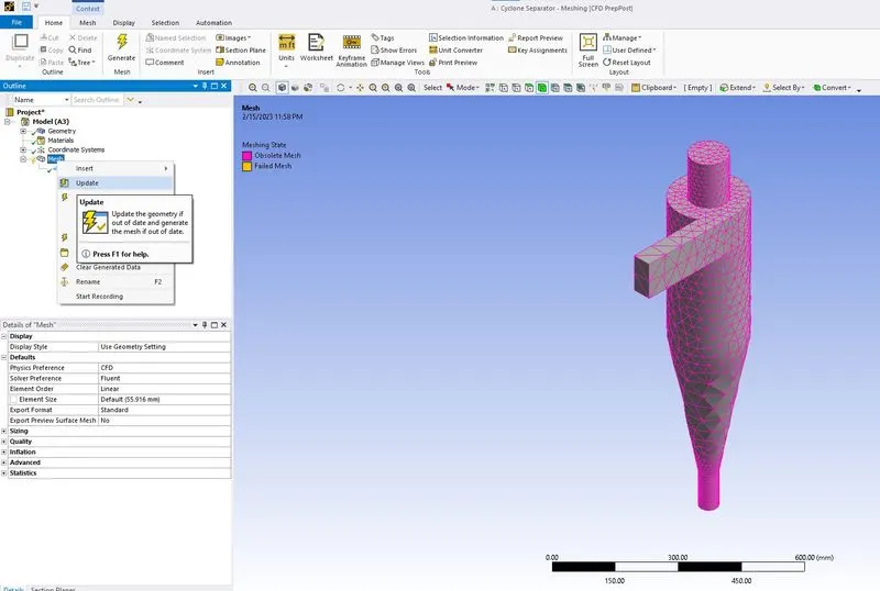
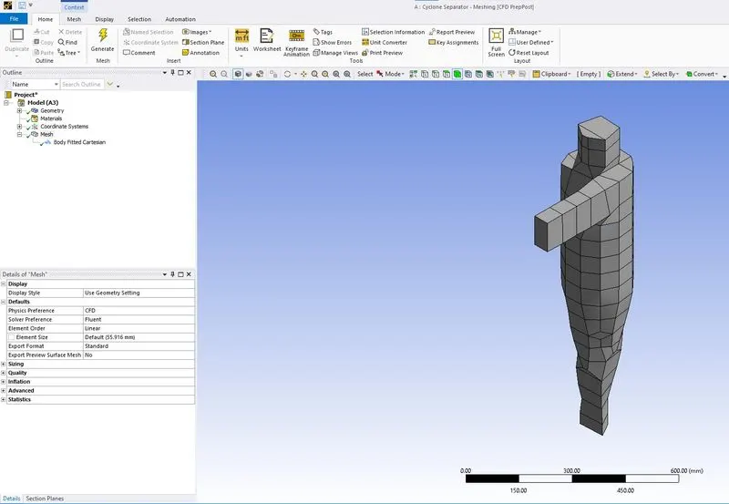
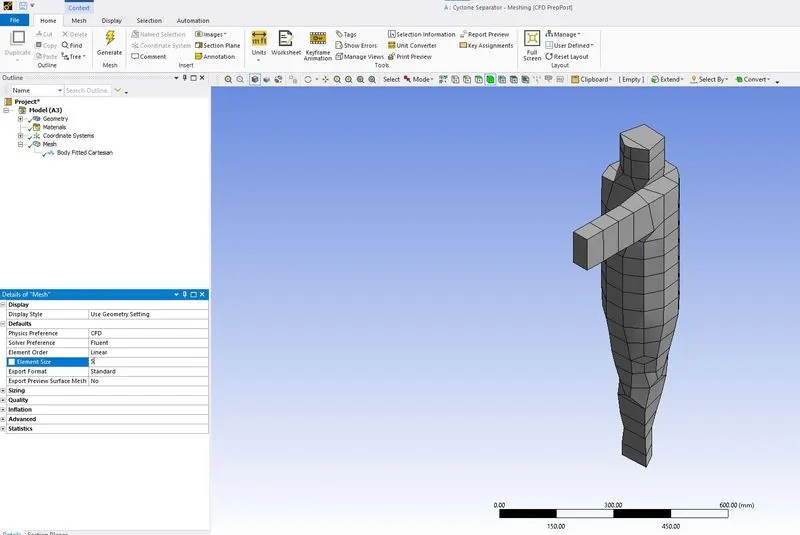
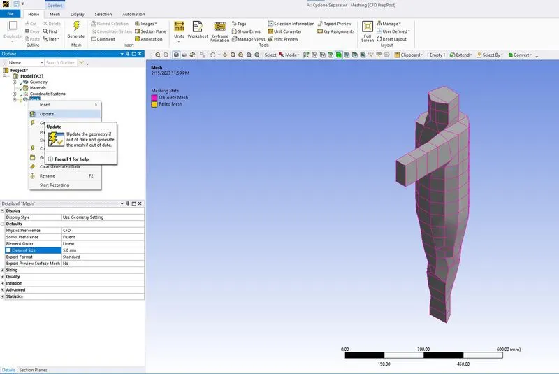
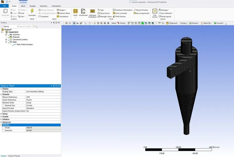
The preview of the final mesh along with the nodes and elements.

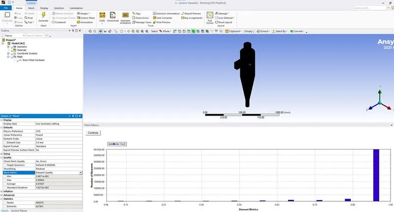
Element quality as shown in the above image.

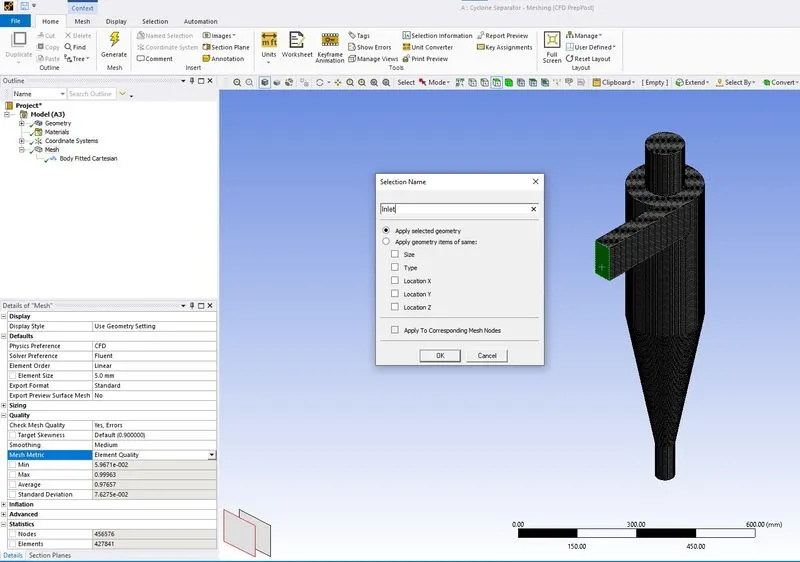
Using the Named selection the selected face is named as Inlet.

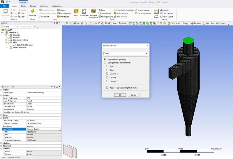
Using the Named selection the selected face is named as Outlet.

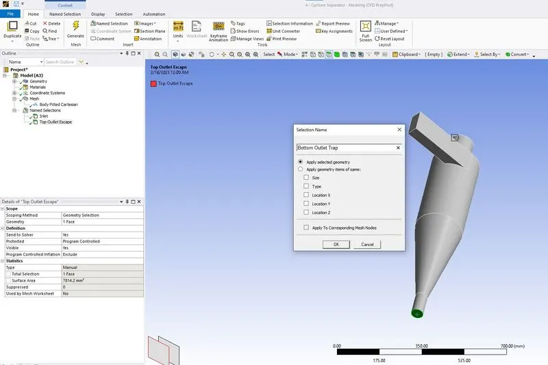
Using the Named selection the selected face is named as Bottom Outlet Trap.

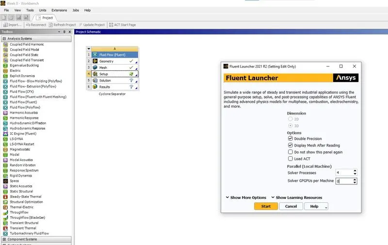
Ansys Fluent set up is opened as shown in the above image.

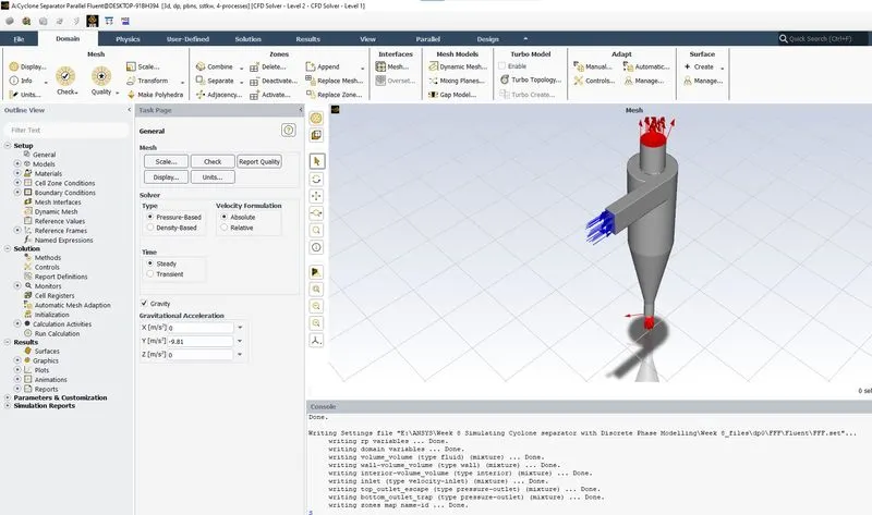
Gravity is enabled as shown in the above image.

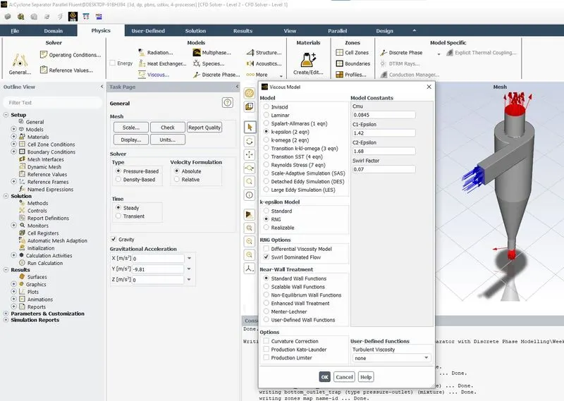
Viscous model is defined as k-epsilon, RNG Method (RNG option as Swirl Dominated Flow) and Near wall treatment as Standard wall functions.

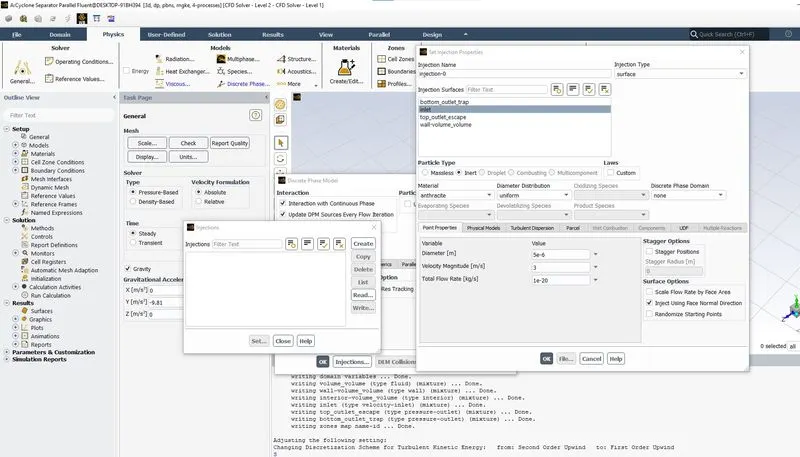
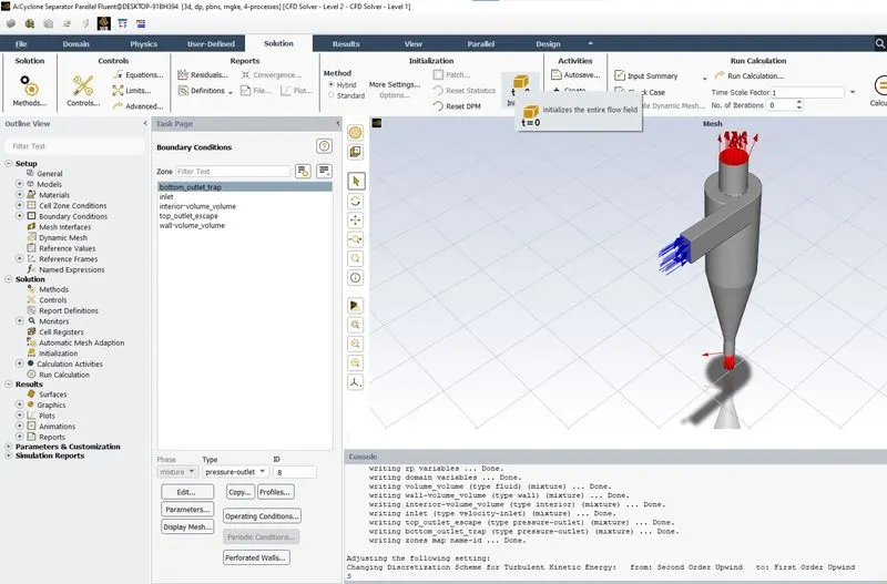
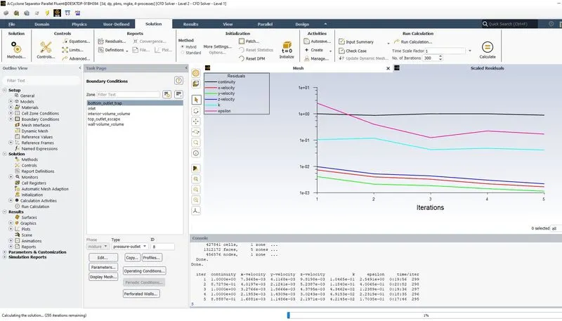
Disscrete phase model is defined as shown in the above image.

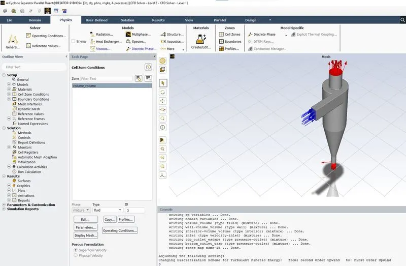
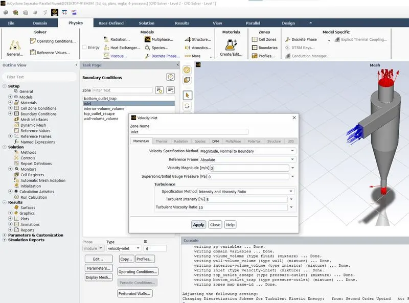
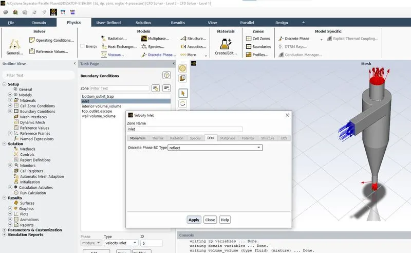
CASE 1: CYCLONE SEPARATOR 1 micrometer 3m/s

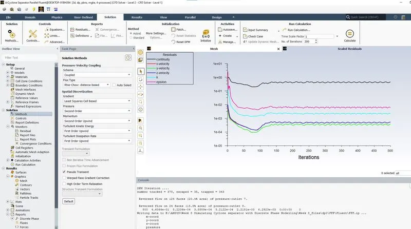
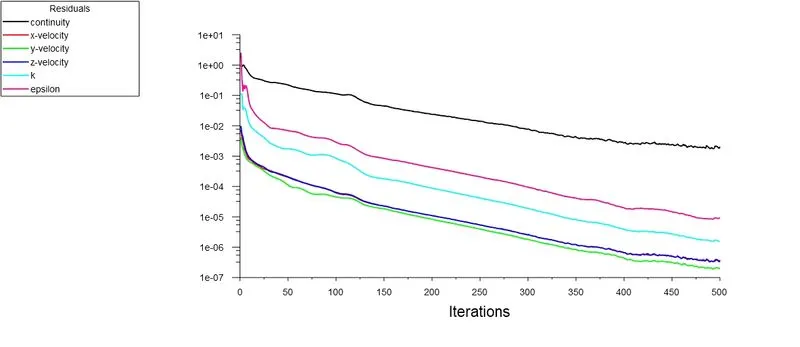
1.1 Scaled Residuals

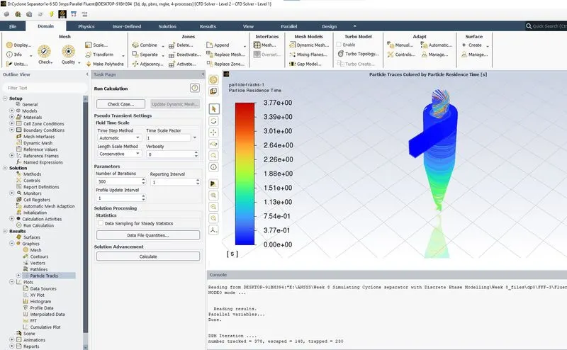
1.2 Particle Residence Time

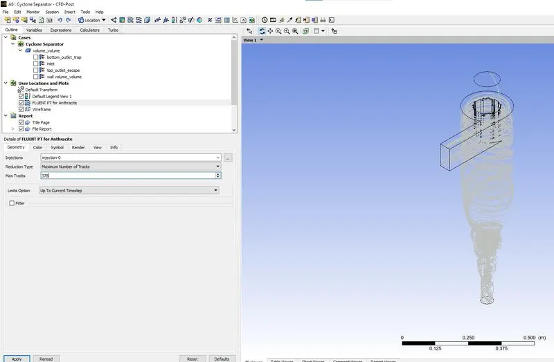
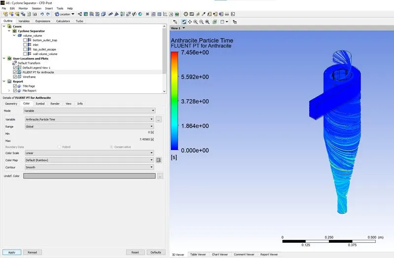
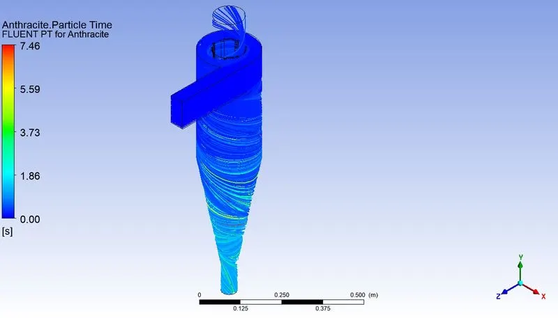
1.3 Antracite Particle Time

1.4 Pressure Contour YZ Plane Centre

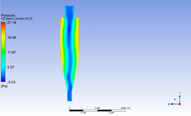
1.5 Pressure Contour YZ Plane Offset near Entry

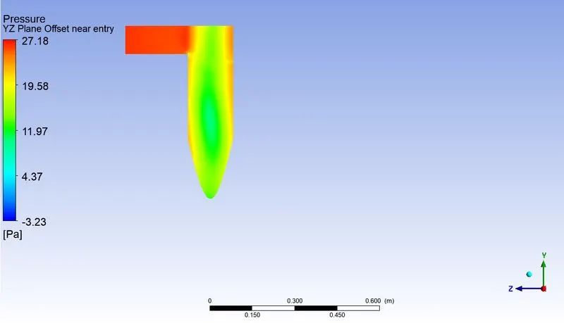
1.6 Velocity Contour YZ Plane Centre

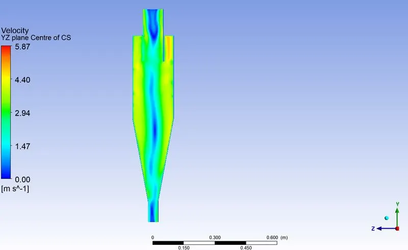
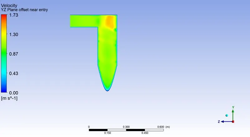
1.7 Velocity Contour YZ Plane Offset near Entry

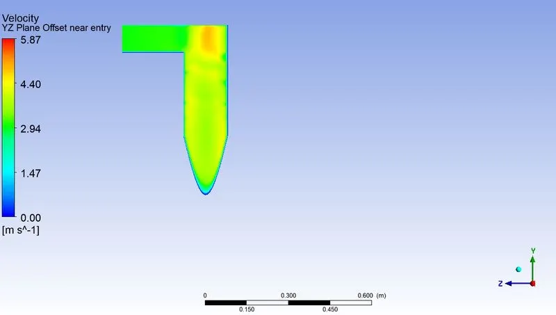
CASE 2: CYCLONE SEPARATOR 3 micrometer 3m/s

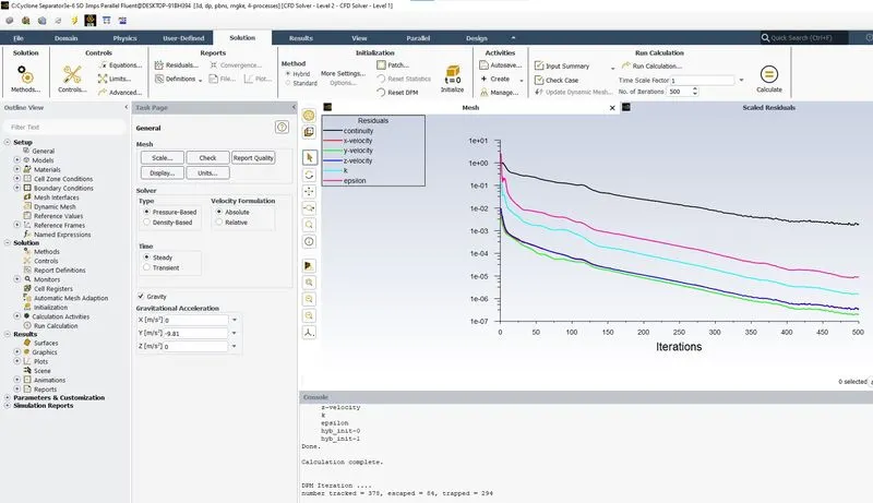
2.1 Scaled Residuals

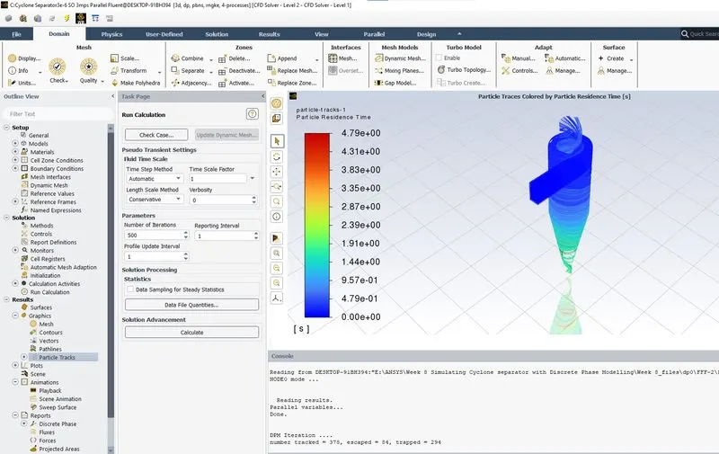
2.2 Particle Residence Time

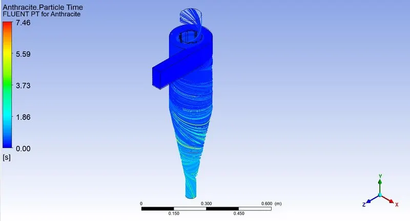
2.3 Antracite Particle Time

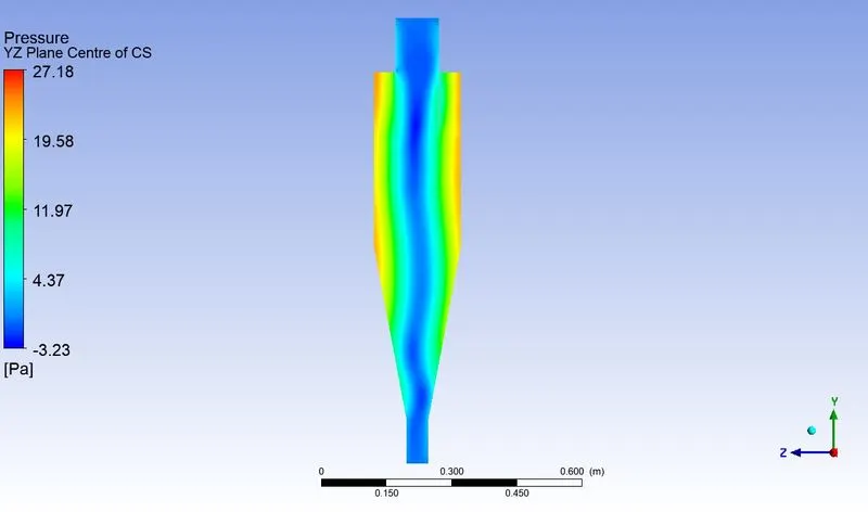
2.4 Pressure Contour YZ Plane Centre

2.5 Pressure Contour YZ Plane Offset near Entry

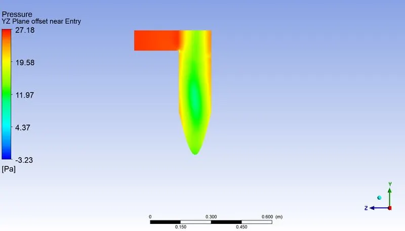
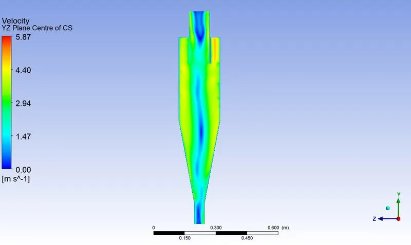
2.6 Velocity Contour YZ Plane Centre

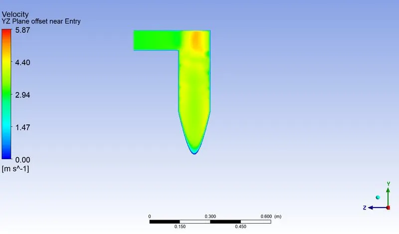
2.7 Velocity Contour YZ Plane Offset near Entry

CASE 3: CYCLONE SEPARATOR 5 micrometer 3m/s

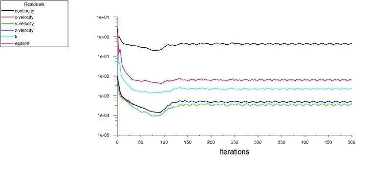
3.1 Scaled Residuals

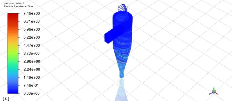
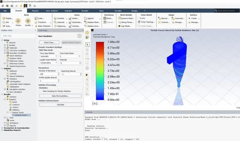
3.2 Particle Residence Time

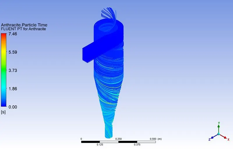
3.3 Antracite Particle Time

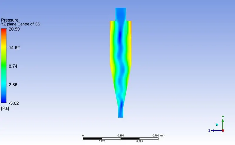
3.4 Pressure Contour YZ Plane Centre

3.5 Pressure Contour YZ Plane Offset near Entry

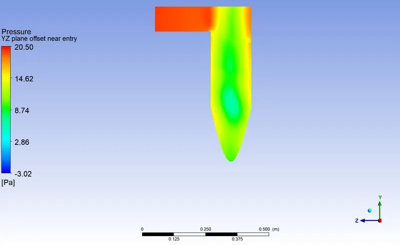
3.6 Velocity Contour YZ Plane Centre

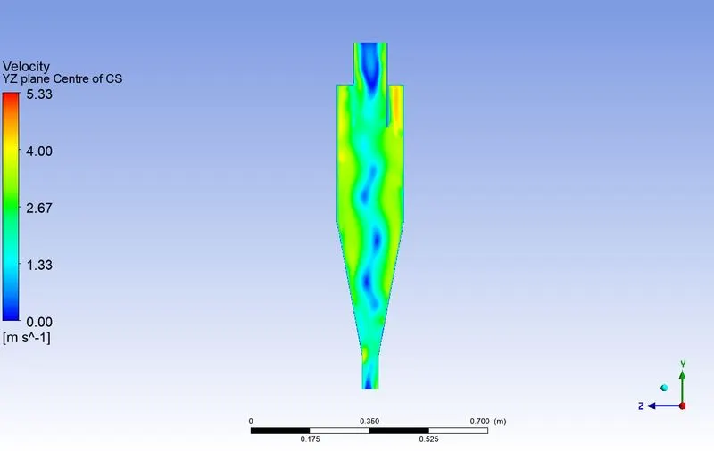
3.7 Velocity Contour YZ Plane Offset near Entry

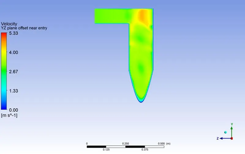
CASE 4: CYCLONE SEPARATOR 5 micrometer 5m/s

4.1 Scaled Residuals

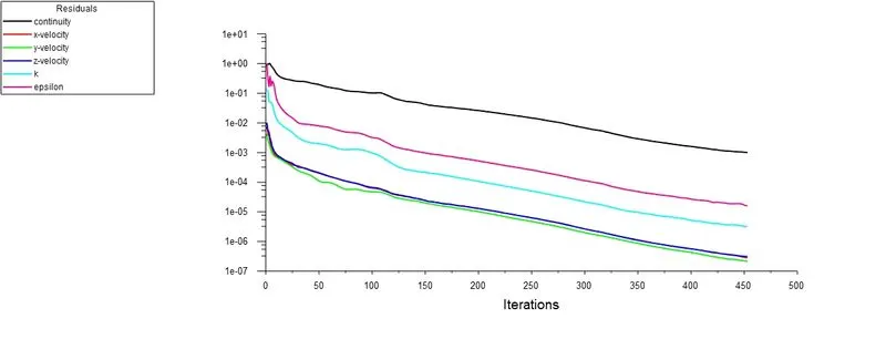
4.2 Particle Residence Time

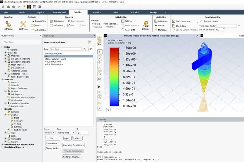
4.3 Antracite Particle Time

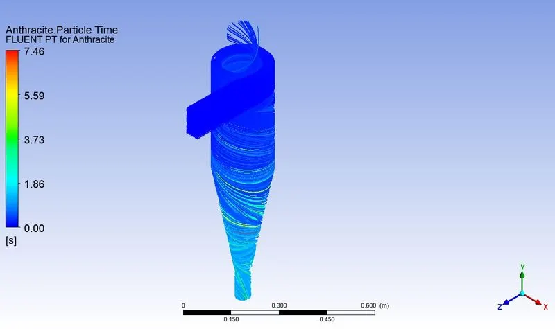
4.4 Pressure Contour YZ Plane Centre

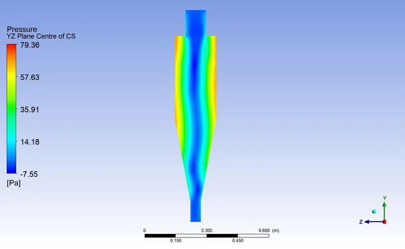
4.5 Pressure Contour YZ Plane Offset near Entry

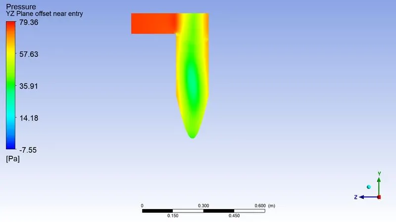
4.6 Velocity Contour YZ Plane Centre

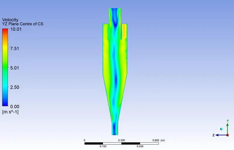
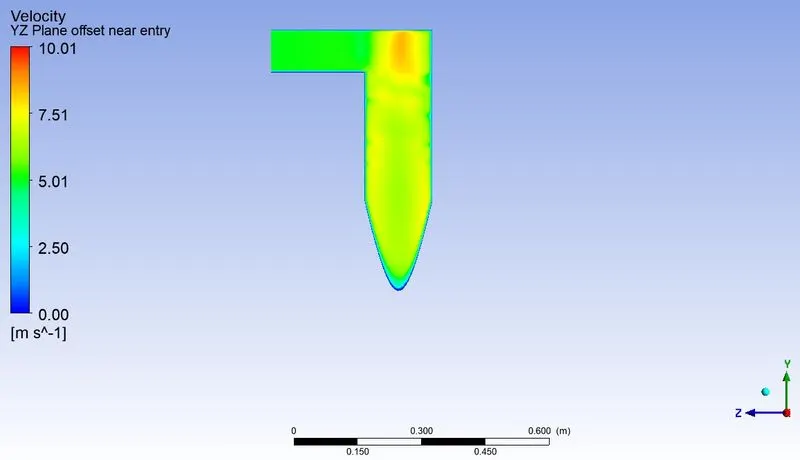
4.7 Velocity Contour YZ Plane Offset near Entry

CASE 5: CYCLONE SEPARATOR 5 micrometer 1m/s

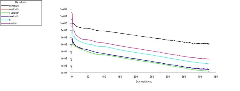
5.1 Scaled Residuals

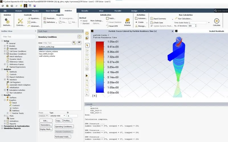
5.2 Particle Residence Time

5.3 Antracite Particle Time

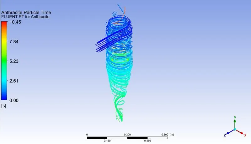
5.4 Pressure Contour YZ Plane Centre

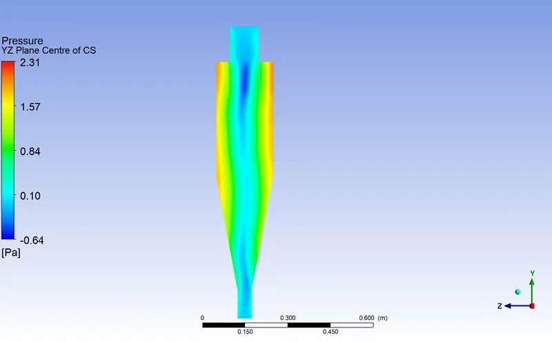
5.5 Pressure Contour YZ Plane Offset near Entry

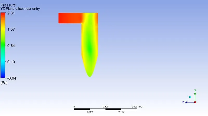
5.6 Velocity Contour YZ Plane Centre

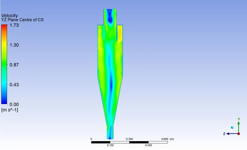
5.7 Velocity Contour YZ Plane Offset near Entry

SEPARATION EFFICIENCY

It is defined as the fraction of particles of a given size collected in the cyclone, compared to those of that size going into the cyclone. Experience shows that the separation efficiency of cyclone separator increases with increasing particle mean diameter and density; increasing gas tangential velocity; decreasing cyclone diameter; increasing cyclone length; extraction of gas along with solids through the cyclone legs.

In this case, depending upon the particle history data - Separation Efficiency is defined as the ratio of concentration that has been removed from the feed stream to the initial concentration in the feed stream. For this case ratio of the number of trapped particles to the total number of particles tracked.

Separation efficiency = no. of particles trapped / no. of particles tracked

PRESSURE DROP

Pressure drop across the cyclone is of much importance in a cyclone separator. The pressure drop significantly affects the performance parameters of a cyclone. The total pressure drop in a cyclone will be due to the entry and exit losses, and friction and kinetic energy losses in the cyclone. Normally the most significant pressure drop occurs in the body due to swirl and energy dissipation.

Pressure drop is defined as the difference in total pressure between two points of a fluid carrying network.

Pressure drop, ΔP = Total inlet pressure - Total Outlet Pressure (escape)

As the escape DPM condition is given to the outlet-top in this case, so outlet-top is considered in pressure drop calculation.

SUMMARY

CONCLUSION:

• The efficiency of a cyclone separator depends on the size and velocity of the particles it is designed to separate. When the particle size is small, the number of particles trapped is more, leading to higher efficiency. However, when the particle size is large, the efficiency decreases.
• The efficiency of a cyclone separator increases with an increase in particle size for constant velocity.
• The efficiency of a cyclone separator increases with an increase in velocity at inlet for constant particle size.
• Pressure drop increases with an increase in inlet velocity for constant particle size..
• Pressure drop in a cyclone separator is caused by the expansion of gas in the cyclone chamber, rotational kinetic energy, and wall frictional forces.