Week 3 - Solving second order ODEs

Simple Pendulum

The following ODE represents the equation of motion of a simple pendulum with damping

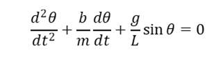
The above equation is a second order ODE.

In the above equation,

g = gravity in m/s2,

L = length of the pendulum in m,

m = mass of the ball in kg,

b=damping coefficient.

The above second order ODE is converted to first order ODE by the following method:

Assume

Differentiating equation '1' with respect to time 't' we get the following

Differentiating equation '2' with respect to time 't' we get the following

Substituting the above equations '1' , '2' & '3' in 'A' we get the following

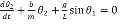
From the equation '2' and '4' we get the following

The above calculation forms the basis for the following function written in MATLAB which will be called in ode45 solver

function [dtheta_dt] = ode_function(t,theta,b,g,l,m)
theta1 = theta(1)
theta2 = theta(2)
dtheta1_dt = theta2;
dtheta2_dt = -(b/m)*theta2 - (g/l)*sin(theta1);
dtheta_dt =[dtheta1_dt; dtheta2_dt];
end

The main code / program written in MATLAB is as follows

clear variables
close all
clc

%Inputs
b=0.05; %Damping Coefficient
g=9.81; %Acceleration due to gravity in m/s^2
l=1;    %Length of pendulum in m 
m=1;  %Suspended ball's mass in Kg

%Initial condition
disp_angvel = [0;3];

%Time Points
t_span = linspace(0,20,500);

%Solve ODE
[t,results] = ode45(@(t,theta) ode_function(t,theta,b,g,l,m),t_span,disp_angvel);

%Plotting
figure(1)
plot(t,results(:,1),'linewidth',1.5)
hold on
plot(t, results(:,2),'linewidth',1.5)
axis([0 25 -4 4])
ylabel('Displacement(rad) & Angular Velocity(rad/sec)')
xlabel('Time(sec)')
legend('Displacement variation wrt Time','Angular Velocity variation wrt Time')
hold off

figure(2)
plot(results(:,1),results(:,2))
xlabel('Displacement or Position (rad)')
ylabel('Angular Velocity(rad/sec')
title('Displacement vs Angular Velocity')

%Animation
theta2=results(:,1);
ct=1;
for i=1:length(theta2)
    theta3=theta2(i);
    
    x0=0;
    y0=0;
    
    x1=l*sin(theta3);
    y1=-l*cos(theta3);
    
    figure(3)
    plot([-1 1],[0 0],'linewidth',2)
    hold on
    plot([x0 x1],[y0 y1],'color','r','linewidth',2.5)
    hold on
    plot(x1,y1,'o','markers',20,'markerfacecolor','b')
    hold off
    grid on
    axis([-3 3 -3 1.5])
    xlabel('X-axis')
    ylabel('Y-axis')
    title('Simple Pendulum Animation')
    pause(0.005)
    M(ct)=getframe(gcf);
    ct=ct+1;
end

movie(M)
videofile = VideoWriter('Simple Pendulum.avi','Uncompressed AVI')
open(videofile)
writeVideo(videofile,M)
close(videofile)

Inputs are noted as the form the variables in the function called in the ODE45 solver

Initial conditions which are stated in the problem forms column vector 2 x1 angular displacement & angular velocity

Time points or the t_span is duration for which we are simulating the motion. t_span is row vector

ode45 only works with functions that use two input arguments, t and y. In our case it is [t,results]

However, you can pass in extra parameters by defining them outside the function and passing them in when you specify the function handle.

In our case function handle is ode_function which pass the extra parmeters as defined in the above written MATLAB code to ODE function.

Based on the results obtained from the ODE45 solver which is an inbuilt MATLAB function the following plots are generated which are as follows.

Refer figure 1 for displacement variation and angular velocity variation with respect to time.

Refer figure 2 for Angular Displacement with respect to Angular velocity

For animation of simple pendulum, for loop is used to get the plot for different values of theta which is captured in M(ct). 'ct' is counter which gets incremented and many such plots are evalauted, plotted and captured as a frame.

Once a bunch of frames are captured, then using those frames a movie or animation is created using movie command by plainy the recorded frames

The following is the syntax for VideoWriter function

v = VideoWriter(filename,profile)

v = VideoWriter(filename,profile) additionally applies a set of properties tailored to a specific file format (such as 'MPEG-4' or 'Uncompressed AVI').

In our case it is,

videofile = VideoWriter('Simple Pendulum.avi','Uncompressed AVI')

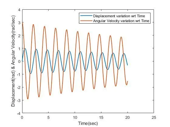
Figure 1 Dispalcement and angular velocity variation with respect to time

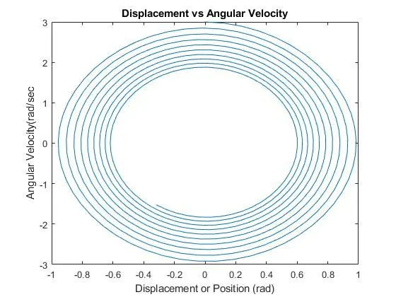
Figure 2 Angular Displacement with respect to Angular velocity

he following logic has been followed for the animation

• For each value in time

Please refer the for loop used in the main code or program

• Create an image that represents the position of the pendulum

x0=0;

y0=0;

x1=l*sin(theta3);

y1=-l*cos(theta3);

plot([x0 x1],[y0 y1],'color','r','linewidth',2.5)

• You can assume the length of the string and the size of the ball

Please refer he inputs used in the program

• Use the marker command to create a sphere

plot(x1,y1,'o','markers',20,'markerfacecolor','b')

• One end of the pendulum is fixed

plot([-1 1],[0 0],'linewidth',2)

• The other end moves according to the solution of the ODE you had solved.

If you are using using Matlab, use the movie command create an animation

movie(M)

videofile = VideoWriter('Simple Pendulum.avi','Uncompressed AVI')

open(videofile)

writeVideo(videofile,M)

close(videofile)

The following video is the animation for simple pendulum

The following error was encountered

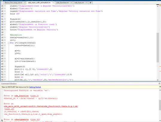
'si' was changed to 'sin'