Otto Engine Cycle

The following code is written in MATLAB to create a PV Diagram of Otto Engine Cycle

Inputs are as follows

gamma is 1.4 for air

Temperature at State3 is t3=2300K

Pressure at State1 is p1=1atm=101325Pa

Temperature at State1 is t1=500K

Engine Geometric Parameters are bore=0.1m, stroke=0.1m, con_rod=0.15m,cr=12

Based on the engine geometric parameters, swept volume and clearance volume are calculated

v1 is the summation of swept volume and clearance volume

v2 is the clearance volume

Based on the above known parameters, the different State variables at different State points are calculated.

clear variables
close all
clc

%Inputs
gamma=1.4
t3=2300 %Temperature at State3 is 2300K

%State variables at State Point 1
p1=101325 %Pressure at State1 is 1atm = 101325Pa
t1=500 %Temperature at State1 is 500K

%Engine Geometric Parameters
bore=0.1;
stroke=0.1;
con_rod=0.15;
cr=12;

%Calculating the swept volume and the clearance volume
v_swept=(pi/4)*bore^2*stroke;
v_clearance=v_swept/(cr-1);

v1=v_swept+v_clearance
v2=v_clearance

%State variables at State Point 2
%p2v2^gamma = p1v1^gamma
%p2=p1*(v1/v2)^gamma=p1*cr^gamma;
p2=p1*cr^gamma;

%p1v1/t1=p2v2/t2 | t2=p2*v2*t1/(p1*v1)
t2=p2*v2*t1/(p1*v1);

constant_c=p1*v1^gamma;
V_Compression=Eng_kin_fu(bore,stroke,con_rod,cr,0,180);

P_Compression=constant_c./V_Compression.^gamma;

%State variables at State Point 3
v3=v2

%p3v3/t3=p2v2/t2 | p3=p2*t3/t2
p3=p2*t3/t2

constant_c=p3*v3^gamma;
V_Expansion=Eng_kin_fu(bore,stroke,con_rod,cr,0,180);

P_Expansion=constant_c./V_Expansion.^gamma;


%State variables at State Point 4
v4=v1

%p3v3^gamma=p4v4^gamma | p4=p3*(v3/v4)^gamma
p4=p3*(v3/v4)^gamma

%Calculating the Thermal Efficiency of the engine
a1=1/(cr^(gamma-1));
eta_thermal=1-a1
fprintf('The thermal efficiency of the engine is %f n',eta_thermal)

figure(1)
hold on
plot(v1,p1,'*','color','r')
plot(V_Compression,P_Compression)
plot(v2,p2,'*','color','r')
plot(v3,p3,'*','color','r')
plot(V_Expansion,P_Expansion)
plot(v4,p4,'*','color','r')
plot([v2,v3],[p2,p3],'color','b')
plot([v4,v1],[p4,p1],'color','b')
xlabel('Pressure (Pa)')
ylabel('Volume (m^3)')
title('PV Diagram of an Otto Engine Cycle')

The following function V is created for Isentropic Process and it is called twice in the main code

1) compression stroke (Reversible adiabatic compression of air)

2) expansion stroke (Reversible adiabatic expansion of air)

function[V]=Eng_kin_fu(bore,stroke,con_rod,cr,start_crank,end_crank)

a=stroke/2;
R=con_rod/a;

%Calculating the swept volume(v_s) and the clearance volume (v_c)
v_s=pi/4*bore^2*stroke;
v_c=v_s/(cr-1);

theta=linspace(start_crank,end_crank,100);

term1=0.5*(cr-1);
term2=R+1-cosd(theta);
term3=(R^2-sind(theta).^2).^0.5;

V=(1+term1*(term2-term3)).*v_c;

end

The following output PV Diagram is plotted for an Otto Engine Cycle. (Refer Figure 1)

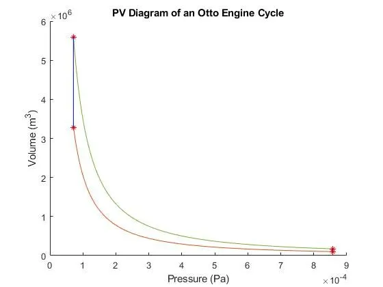
Figure1

The output for thermal efficiency is generated.(Refer Figure 2)

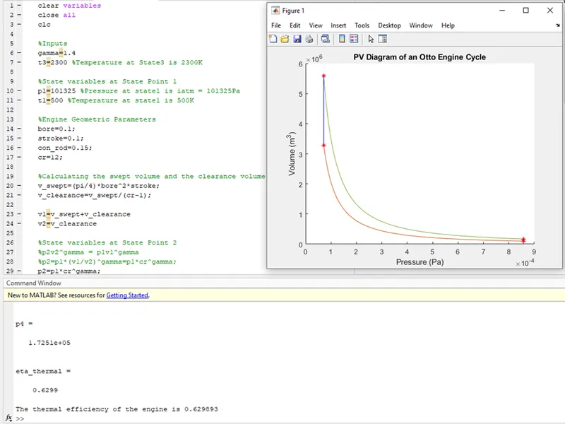
Figure 2

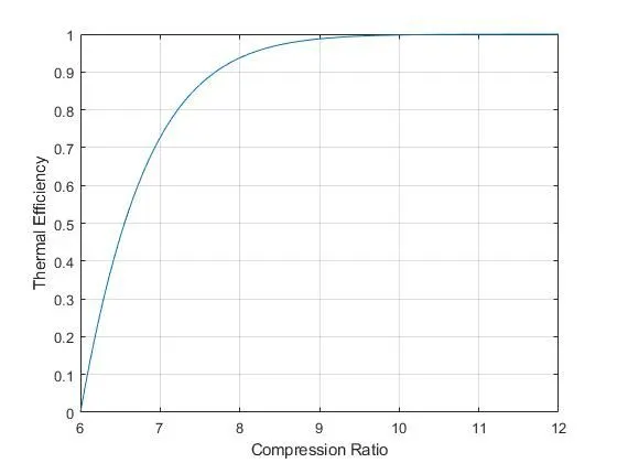
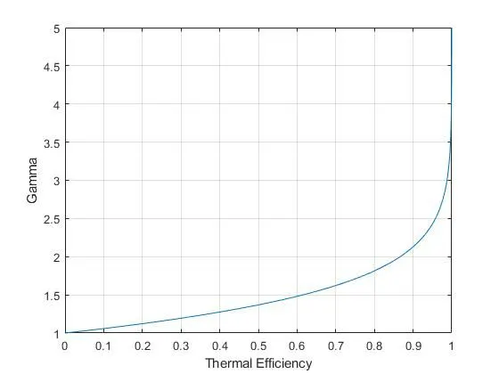
The following code helps us to understand the relattionship between thermal efficiency, compression ratio and gamma

clear variables
close all
clc

gamma=linspace(1,5,100)

cr=linspace(6,12,100)

a1=1./(cr.^(gamma-1));
eta_thermal=1-a1

figure(1)
plot(cr,eta_thermal)
xlabel('Compression Ratio')
ylabel('Thermal Efficiency')
grid on

figure(2)
plot(eta_thermal,gamma)
xlabel('Thermal Efficiency')
ylabel('Gamma')
grid on