Week 8 - Simulating Cyclone separator with Discrete Phase Modelling
Aim:- To perform analysis on cyclone separator and calculate the separation efficiency and pressure drop.
Objective:-
- To write a few words about any four empirical models used to calculate the cyclone separator efficiency.
- To perform an analysis on a given cyclone separator model by varying the particle diameter from 1 μm to 5 μm and calculate the separation efficiency in each case. Discuss the results. [Use both the velocity's as 3m/sec.]
- To perform an analysis on a given cyclone separator model by varying the particle velocity from 1 m/sec to 5 m/sec and calculate the separation efficiency and pressure drop in each case. Discuss the results. [Use particle diameter size as 5 μm for all cases & keep flow velocity same as particle velocity]
Boundary Conditions:-
Inlet and wall:- Reflect
Outlet(Top):- Escape
Outlet(Bottom/dustbin) - Trap
Introduction :-
Cyclonic separation is a method of removing particulates from an air, gas or liquid stream, without the use of filters, through vortex separation. When removing particulate matter from liquid, a hydrocyclone is used; while from gas, a gas cyclone is used. Rotational effects and gravity are used to separate mixtures of solids and fluids. The method can also be used to separate fine droplets of liquid from a gaseous stream.
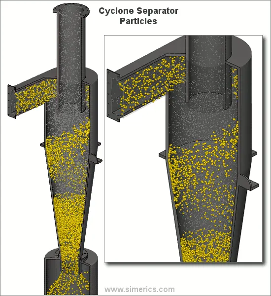
A high speed rotating (air)flow is established within a cylindrical or conical container called a cyclone. Air flows in a helical pattern, beginning at the top (wide end) of the cyclone and ending at the bottom (narrow) end before exiting the cyclone in a straight stream through the center of the cyclone and out the top. Larger (denser) particles in the rotating stream have too much inertia to follow the tight curve of the stream, and thus strike the outside wall, then fall to the bottom of the cyclone where they can be removed. In a conical system, as the rotating flow moves towards the narrow end of the cyclone, the rotational radius of the stream is reduced, thus separating smaller and smaller particles. The cyclone geometry, together with volumetric flow rate, defines the cut point of the cyclone. This is the size of particle that will be removed from the stream with a 50% efficiency. Particles larger than the cut point will be removed with a greater efficiency, and smaller particles with a lower efficiency as they separate with more difficulty or can be subject to re-entrainment when the air vortex reverses direction to move in direction of the outlet.
Working principle :-
Product is fed into the cyclone seperator tangentially under a certain pressure. This creates a centrifugal movement, pushing the heavier phase outward and downward alongside the wall of the conical part. The decreasing diameter in the conical part increases the speed and so enhances the separation. Finally, the concentrated solids are discharged through the apex. The vortex finder in the overflow part creates a fast rotating upward spiral movement of the fluid in the centre of the conically shaped housing. The fluid is discharged through the overflow outlet.
Parameters for good cyclone operation :
The following parameters are decisive for good cyclone operation:
The design.
The specific weight difference between the two product phases.
The shape of the solids.
The speed of the feed.
The density of the medium.
The counter pressure at the overflow and apex.
Empirical models used to calculate the cyclone separator efficiency :-
1) IOZIA AND LEITH MODEL :
Iozia and Leith (1990) logistic model is a modified version of Barth (1956) model which is developed based on force balance. The model assumes that a particle carried by the vortex endures the influence of two forces: a centrifugal force, Z, and a flow resistance, W. Core length, zc , and core diameter, dc , are given as,
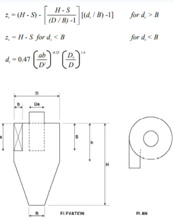
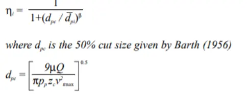
- The addition made by Iozia and Leith on the original Barth (1956) model are the core length zc and slope parameter β expression which is derived based on the statistical analysis of experimental data of cyclone with D = 0.25 m. The collection efficiency ηi of particle diameter dpi can be calculated from.
2) LI AND WANG MODEL :
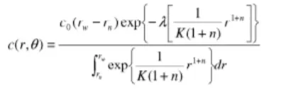
- The Li and Wang (1989) model includes particle bounce or re-entrainment and turbulent diffusion at the cyclone wall. A two-dimensional analytical expression of particle distribution in the cyclone is obtained. Li and Wang model was developed based on the following assumptions:
• The radial particle velocity and the radial concentration profile are not constant, for uncollected particles within the cyclones.
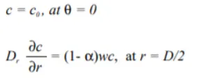
• Boundary conditions with the consideration of turbulent diffusion coefficient and particle bounce re-entrainment on the cyclone wall are:
- The tangential velocity is related to the radius of cyclone by: uRn = constant.
- The concentration distribution in a cyclone is given as:
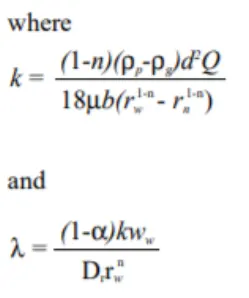
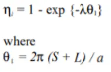
- The resultant expression of the collection efficiency for particle of my size is given as
3) KOCH AND LICHT MODEL :
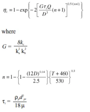
- Koch and Licht (1977) collection theory recognized the inherently turbulent nature of cyclones and the distribution of gas residence times within the cyclone. Koch and Licht describe particle motion in the entry and collection regions with the additional following assumptions:
• The tangential velocity of a particle is equal to the tangential velocity of the gas flow, i.e. there is no slip in the tangential direction between the particle and the gas.
• The tangential velocity is related to the radius of cyclone by: uRn = constant. - A force balance and an equation on the particles collection yields the grade efficiency η_i.
4) LAPPLE MODEL :
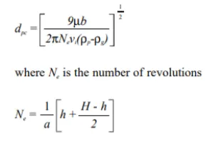
- Lapple (1951) model was developed based on force balance without considering the flow resistance. Lapple assumed that a particle entering the cyclone is evenly distributed across the inlet opening. The particle that travels from inlet half width to the wall in the cyclone is collected with 50% efficiency. The semi empirical relationship developed by Lapple (1951) to calculate a 50% cut diameter, dpc, is,
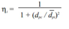
- The efficiency of collection of any size of particle is given by
The cyclone efficiency predicted by the Li and Wang model is very accurate at room temperature. The experimental results from the Ray's and Kim and Lee's studies are more closely fit by the Li and Wang model. The Lapple, Koch, and Licht models have a significant overestimation of efficiency for tiny particles and a significant underestimation of efficiency for big particles. The logistic model developed by Iozia and Leith exhibits good agreement with experimental data for cyclones with diameters between 0.25 and 0.4 meters. It cannot, however, accurately forecast the efficiency of minor cyclones (D 0.1m). Only cyclones with diameters about 0.25 m can be efficiently predicted using the Iozia and Leith model. When severe conditions, such as extremely high temperatures and pressure, are present, the Lapple model exhibits a reasonable.
Solution procedure :-
We will simulate by using DPM .Let us first discuss about discrete Phase Modelling.
Discrete Phase Modelling (DPM) :
The Lagrangian discrete phase model in ANSYS FLUENT follows the Euler-Lagrange approach. The fluid phase is treated as a continuum by solving the Navier-Stokes equations, while the dispersed phase is solved by tracking a large number of particles, bubbles, or droplets through the calculated flow field. The dispersed phase can exchange momentum, mass, and energy with the fluid phase.
A fundamental assumption made in this model is that the dispersed second phase occupies a low volume fraction(<10%). The particle or droplet trajectories are computed individually at specified intervals during the fluid phase calculation.
ANSYS FLUENT predicts the trajectory of a discrete phase particle (or droplet or bubble) by integrating the force balance on the particle, which is written in a Lagrangian reference frame. This force balance equates the particle inertia with the forces acting on the particle .
We wil simulate all the 6 cases with steady state. For solving we follow the below procedure :
1)Geometry setup
2)Meshing
3) Problem setup
4)Solving
5)Post processing
Performing an analysis on cyclone separator model by varying the particle diameter from 1 μm to 5 μm. (We use both the flow and particle velocity as 3m/sec) :
Here we perform an analysis on a given cyclone separator model by varying the particle diameter from 1 μm to 5 μm and calculate the separation efficiency in each case and discuss the results.Here we use both the flow velocity and particle velocity as 3m/sec.
Let us perform the simulation for each case by following the above procedure.
Case 1 :-
Particle diameter of 1 μm :
Geometry setup :
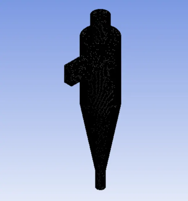
In fluent module we have to open spaceClaim and then import the 3D geometry.The below image is the 3D view of cyclone separator.
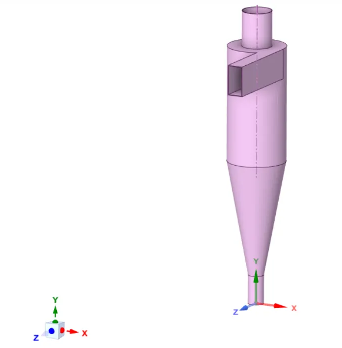
Here the outlet at the bottom is for heavier particles and the light particles will come out of the outlet at the top.
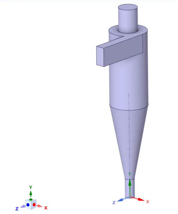
We need to extract the fluid volume first.For that ,
steps : prepare -> volume extract -> select the fluid volume by selecting the edges of inlet and 2 outlets -> Then ok.
Then new object will be added to the tree.Then hide the solid volume and suppress it for physics and the left is fluid volume which we generated.
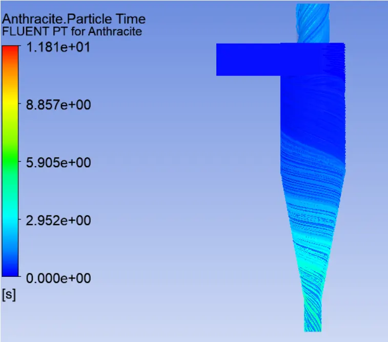
Anthracite particle time contour :
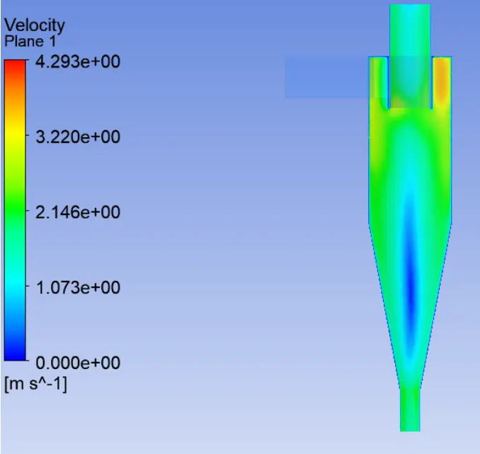
Velocity contour :
- In the below image we can see the velocity contour on the midplane of cyclone separator .
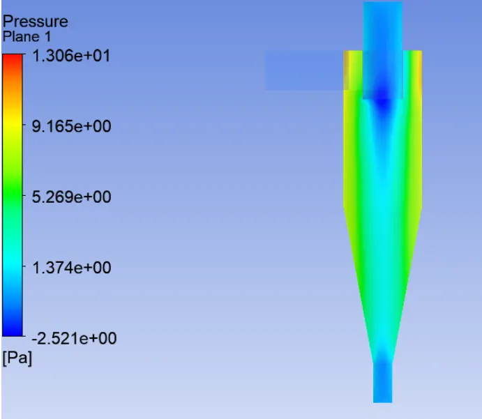
Pressure contour :
- In the below image we can see the pressure contour on the midplane of cyclone separator.
Residual Plot:
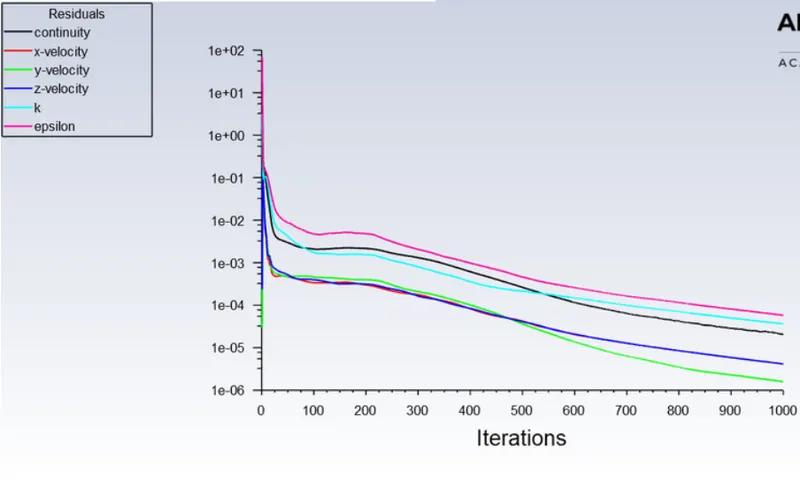
Case 2 :-
Particle diameter of 3 μm :
Everything is same as previous case from the point of geometry and mesh.
Comming to set up the only change here is in the injections in the discrete phase modelling we give particle dia meter as 3 μm .Remaining everything is same as previous case.
Then we run for 1000 iterations .
So let us directly run the simulation and then post process the results.
Post processing :
Then open CFD post and import the results for that,
Open results -> Import the data by selecting file -> then select import -> then select import fluent particle track file -> Then open newly saved file .
Then you can see fluent PT for anthracite file after import .Then double click on that you can give maximum number of particles to display ,as we have tracked 372 particles let us give 372.
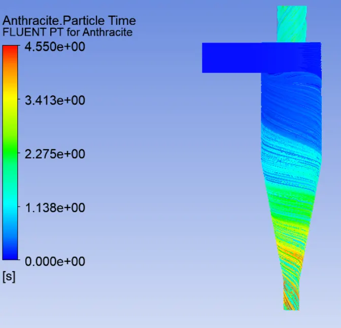
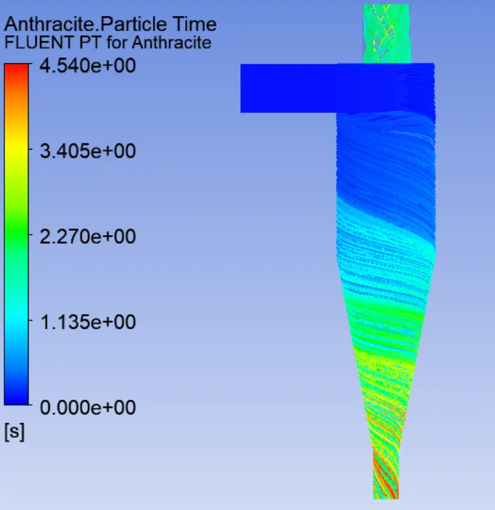
Then let us colour particle track by the anthracite particle time, which shows the residence time of each particle.
Anthracite particle time contour :
Velocity contour :
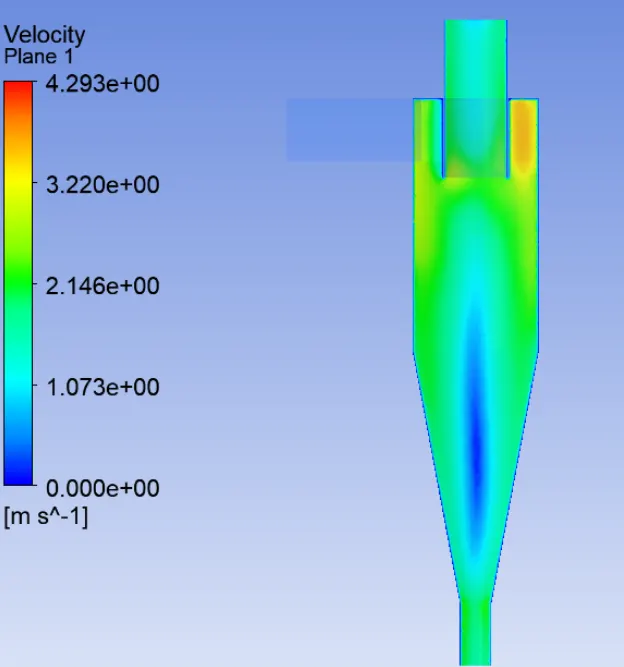
- In the below image we can see the velocity contour on the midplane of cyclone separator .
Pressure contour :
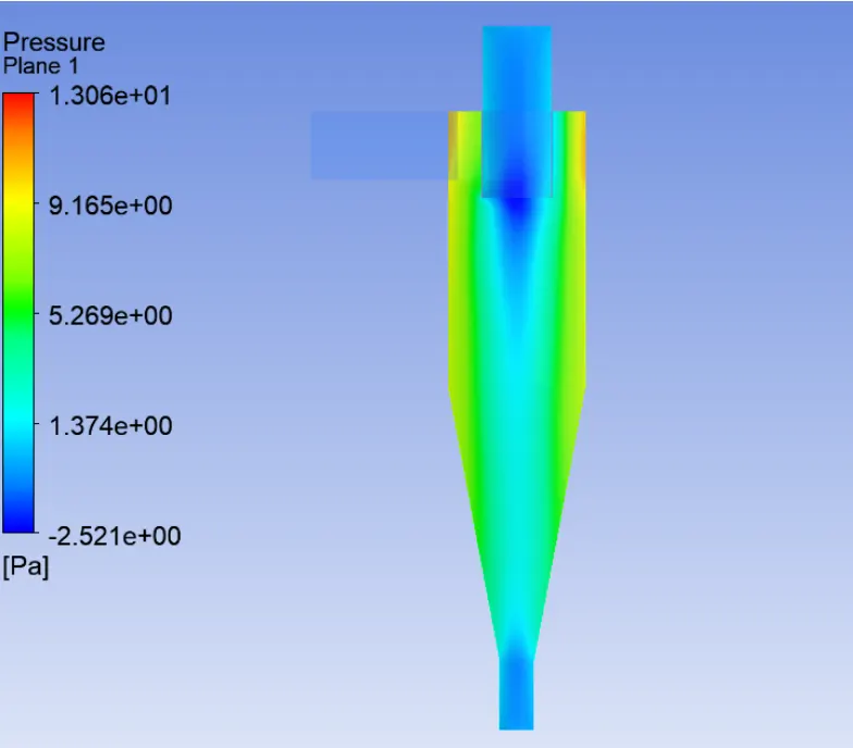
- In the below image we can see the pressure contour on the midplane of cyclone separator
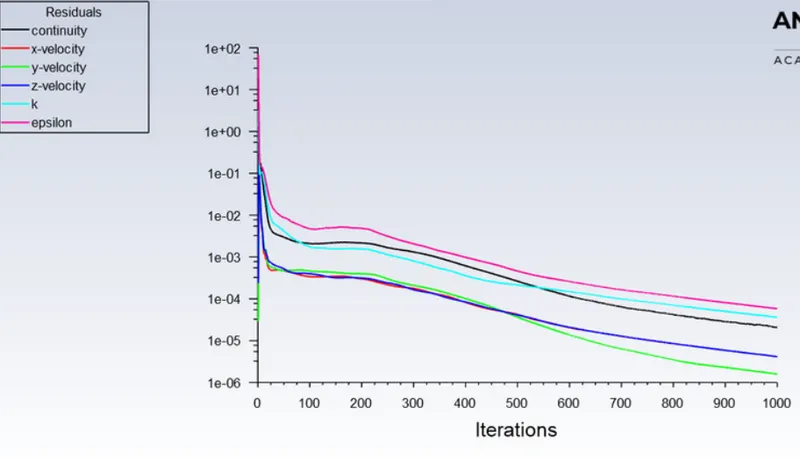
Residual plot:
Case 3 :-
Particle diameter of 5 μm :
Everything is same as previous case from the point of geometry and mesh.
Comming to set up the only change here is in the injections in the discrete phase modelling we give particle dia meter as 5 μm .Remaining everything is same as previous case.
Then we run for 1000 iterations .
So let us directly run the simulation and then post process the results.
Post processing :
Then open CFD post and import the results for that,
Open results -> Import the data by selecting file -> then select import -> then select import fluent particle track file -> Then open newly saved file .
Then you can see fluent PT for anthracite file after import .Then double click on that you can give maximum number of particles to display ,as we have tracked 372 particles let us give 372.
Then let us colour particle track by the anthracite particle time, which shows the residence time of each particle.
Anthracite particle time contour :
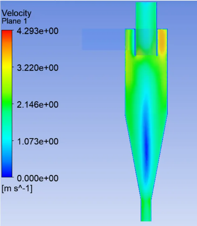
Velocity contour :
- In the below image we can see the velocity contour on the midplane of cyclone separator .
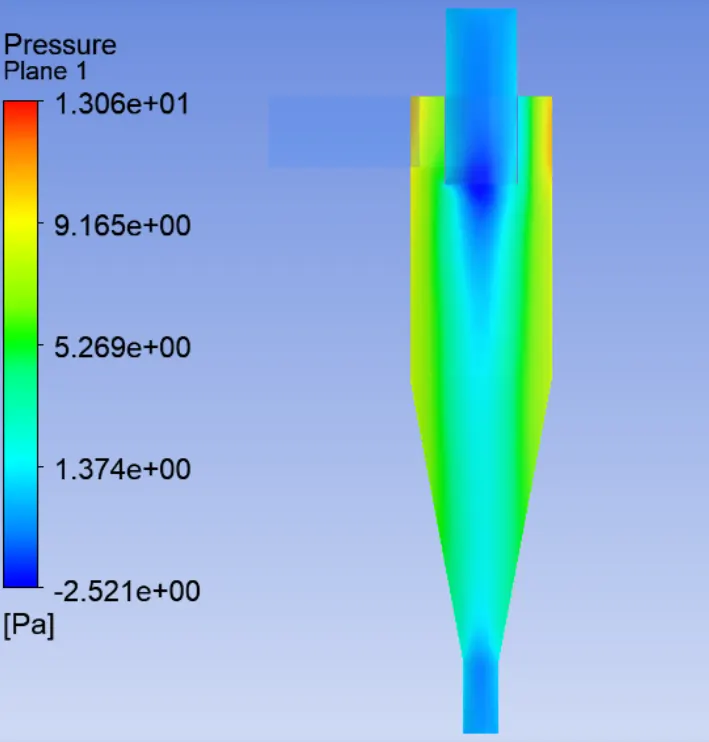
Pressure contour :
- In the below image we can see the pressure contour on the midplane of cyclone separator
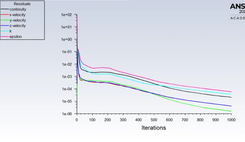
Residuals plot :
Conclusions:-
If you look at the above table, you can see that when the particle diameter rises, there are more particles trapped at the bottom output, which likewise raises the cyclone separator's separation effectiveness.
You can detect some unfinished particles that struck in the recirculation region when the particle diameter is quite small.
Analyzing the cyclone separator model with a particle velocity range of 1 m/sec to 5 m/sec:
Here, we analyze a specific cyclone separator model with particle velocities ranging from 1 m/s to 5 m/s, and we determine the separation efficiency and pressure drop in each scenario.
The outcomes are then discussed.
Here, we maintain the same flow velocity and use a particle diameter size of 5 m in all scenarios.
Case 1 :-
Particle velocity of 1 m/sec :
Everything is same as previous case from the point of geometry and mesh.
Comming to set up the changes here is in the injections in the discrete phase modelling we give particle dia meter as 5 μm and here we keep flow velocity same as particle velocity = 1 m/sec remaining everything is same as previous case.
Then we run for 1000 iterations .
So let us directly run the simulation and then post process the results.
Post processing :
Then open CFD post and import the results for that,
Open results -> Import the data by selecting file -> then select import -> then select import fluent particle track file -> Then open newly saved file .
Then you can see fluent PT for anthracite file after import .Then double click on that you can give maximum number of particles to display ,as we have tracked 372 particles let us give 372.
Then let us colour particle track by the anthracite particle time, which shows the residence time of each particle.
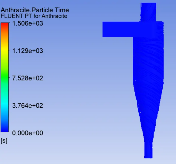
Anthracite particle time contour :
- Anthracite particle time contour for 372 particles.
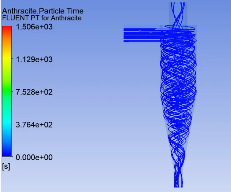
- For better visualization of anthracite particle time contour , let us give particle count as 25 particles.
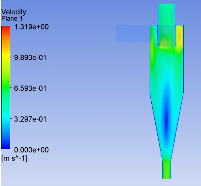
Velocity contour :
- In the below image we can see the velocity contour on the midplane of cyclone separator .
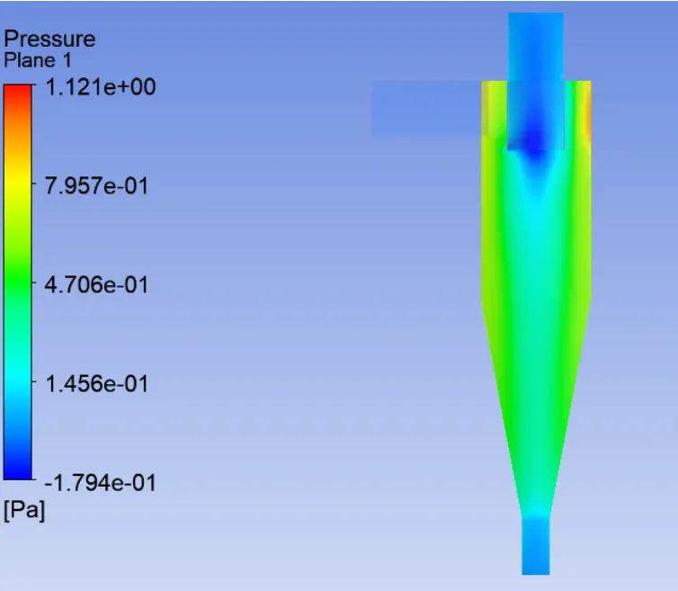
Pressure contour :
- In the below image we can see the pressure contour on the midplane of cyclone separator
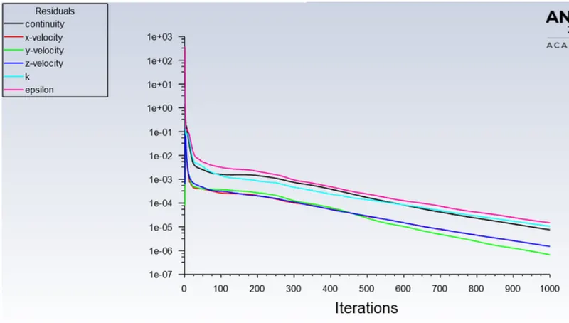
Residuals plot :
Case 2 :-
Particle velocity of 3 m/sec :
Everything is same as previous case from the point of geometry and mesh.
Comming to set up the changes here is in the injections in the discrete phase modelling we give particle diameter as 5 μm and here we keep flow velocity same as particle velocity = 3 m/sec remaining everything is same as previous case.
Then we run for 1000 iterations .
So let us directly run the simulation and then post process the results.
Post processing :
Then open CFD post and import the results for that,
Open results -> Import the data by selecting file -> then select import -> then select import fluent particle track file -> Then open newly saved file .
Then you can see fluent PT for anthracite file after import .Then double click on that you can give maximum number of particles to display ,as we have tracked 372 particles let us give 372.
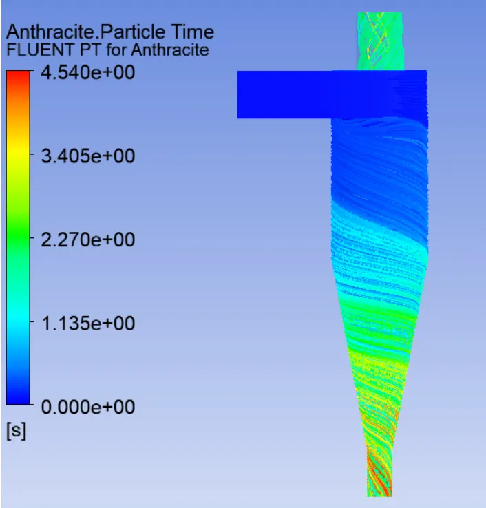
Then let us colour particle track by the anthracite particle time, which shows the residence time of each particle.
Anthracite particle time contour :
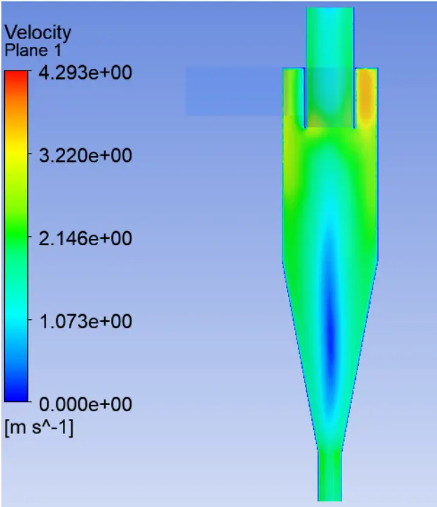
Velocity contour :
- In the below image we can see the velocity contour on the midplane of cyclone separator .
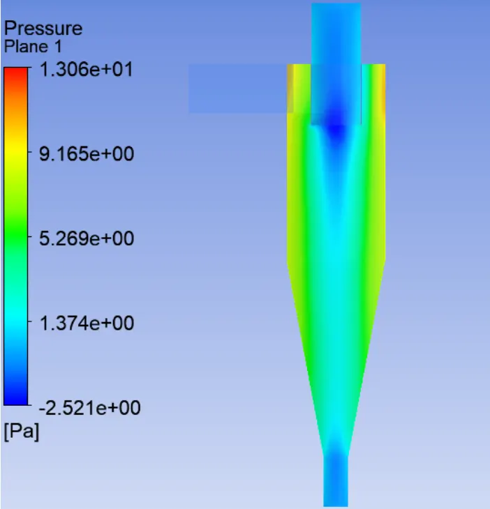
Pressure contour :
- In the below image we can see the pressure contour on the midplane of cyclone separator
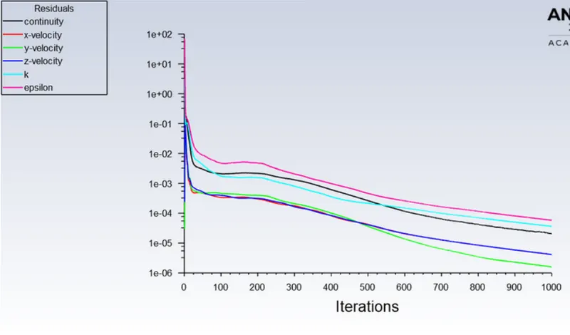
Residuals plot :
Case 3 :-
Particle velocity of 5 m/sec :
Everything is same as previous case from the point of geometry and mesh.
Comming to set up the changes here is in the injections in the discrete phase modelling we give particle diameter as 5 μm and here we keep flow velocity same as particle velocity = 5 m/sec remaining everything is same as previous case.
Then we run for 1000 iterations .
So let us directly run the simulation and then post process the results.
Post processing :
Then open CFD post and import the results for that,
Open results -> Import the data by selecting file -> then select import -> then select import fluent particle track file -> Then open newly saved file .
Then you can see fluent PT for anthracite file after import .Then double click on that you can give maximum number of particles to display ,as we have tracked 372 particles let us give 372.
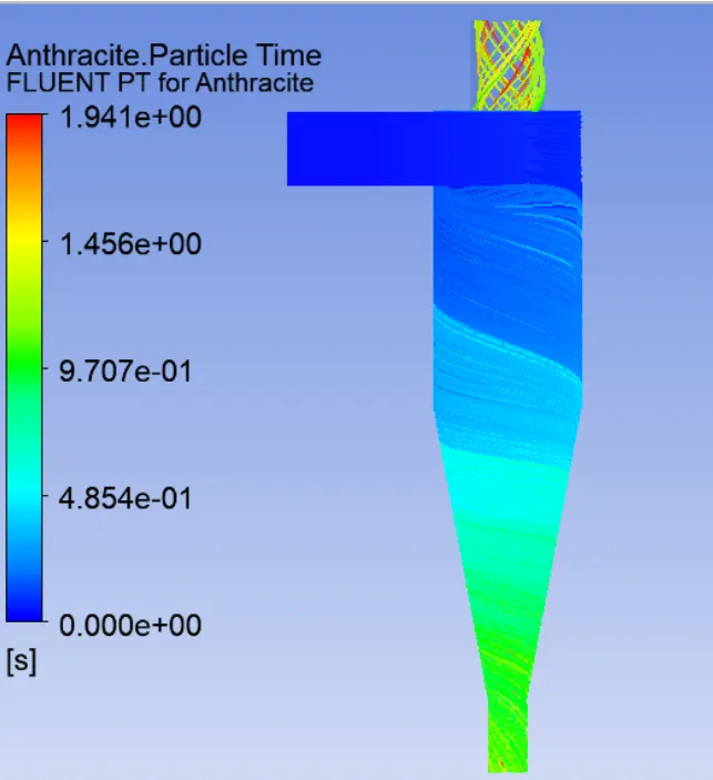
Then let us colour particle track by the anthracite particle time, which shows the residence time of each particle.
Anthracite particle time contour :
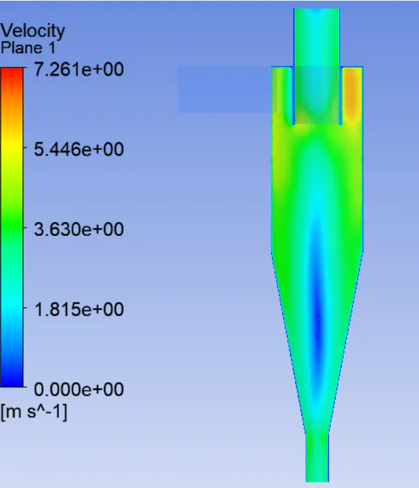
Velocity contour :
- In the below image we can see the velocity contour on the midplane of cyclone separator .
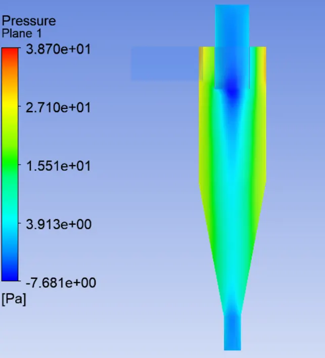
Pressure contour :
- In the below image we can see the pressure contour on the midplane of cyclone separator
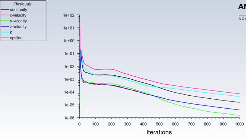
Residuals plot :
Conclusions:-
Numerical study of gas–solid flow in a cyclone separator,
Applied Mathematical Modelling,
Volume 30, Issue 11,
2006,
Pages 1326-1342.