Week 8 - Simulating Cyclone separator with Discrete Phase Modelling

Aim:-

 To perform analysis on cyclone separator and calculate the separation efficiency and pressure drop.  

Objective:-

1. To write a few words about any four empirical models used to calculate the cyclone separator efficiency. 
2. To perform an analysis on a given cyclone separator model by varying the particle diameter from 1 μm to  5 μm and calculate the separation efficiency in each case. Discuss the results. [Use both the velocity's as 3m/sec.]
3. To perform an analysis on a  given cyclone separator model by varying the particle velocity from 1 m/sec to 5 m/sec and calculate the separation efficiency and pressure drop in each case. Discuss the results. [Use particle diameter size as 5 μm for all cases & keep flow velocity same as particle velocity]

Boundary Conditions:-

Inlet and wall:- Reflect

Outlet(Top):- Escape 

Outlet(Bottom/dustbin) - Trap

Discrete phase modelling:

It is a type of multiphase modelling where there is a presence of different phase particles on continous phase.

eg. applications such as cyclone seperator ; fuel injectors in automobiles.

Cyclone seperator:

Cyclone separator are an economical device for removing particulate solids from a fluid system. Particle along with a working fluid gets introduced via a stream through inlet, the induced centrifugal force is tangentially imparted on the wall of the cyclone cylinder. This force, with the density difference between the fluid and solid, increases the relative settling velocity. The heavier particle tends to slid down and are trapped in the lower outlet pane. Though the cyclone separator are highly efficient, but its efficiency varies given the particle size and flow velocity. The particles sometimes tend to escape with the working fluid making it less efficient.

emprical models in cyclone seperator efficiency:

1.Iozia and Leith Model :

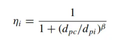
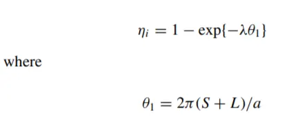
Iozia and Leith  logistic model is a modified version of Barth Model, which is developed based on force balance. The model assumes that a particle carried by the vortex endures  the influence of two forces: a centrifugal force, Z and a flow resistance, W. The collection efficiency η_i of particle diameter d_pi can be calculated from

                                                        

β is an expression for slope parameter derived based on the statistical analysis of experimental data of a cyclone with D = 170 0.25 m given as

                                   

and dpc is the 50% cut size given by Barth

                            

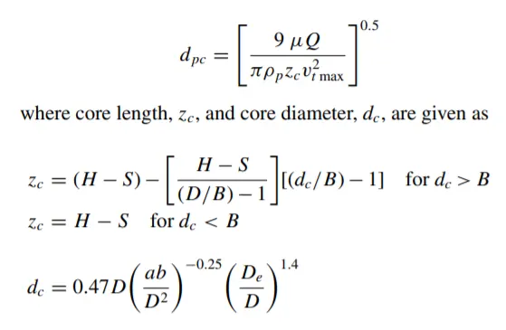
2.Li and Wang Model :

The Li and Wang model includes particle bounce or reentrainment and turbulent diffusion at the cyclone wall. A twodimensional analytical expression of particle distribution in the cyclone is obtained. Li and Wang model was developed based on the following assumptions:

• The radial particle velocity and the radial concentration profile are not constant for uncollected particles within the cyclone.
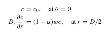
• Boundary conditions with the consideration of turbulent diffusion coefficient and particle bounce reentrainment on the cyclone wall are:

                                                      

• The tangential velocity is related to the radius of cyclone by: uRⁿ = constant.

The concentration distribution in a cyclone is given as:

                                  

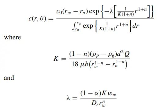
The resultant expression of the collection efficiency for particle of any size is given as

                                       

3.Koch and Licht Model

Koch and Licht  collection theory recognized the inherently turbulent nature of cyclones and the distribution of gas residence times within the cyclone. Koch and Licht described particle motion in the entry and collection regions with the additional following assumptions:

• The tangential velocity of a particle is equal to the tangential velocity of the gas flow, i.e. there is no slip in the tangential direction between the particle and the gas.
• The tangential velocity is related to the radius of cyclone by: uRⁿ = constant.

A force balance and an equation on the particles collection yields the grade efficiency η_i

                                 

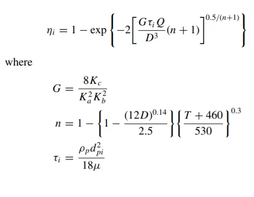
G is a factor related to the configuration of the cyclone, n is related to the vortex and τ is the relaxation term.

4.Lapple Model

Lapple model was developed based on force balance without considering the flow resistance. Lapple assumed that a particle entering the cyclone is evenly distributed across the inlet opening. The particle that travels from inlet half width to the wall in the cyclone is collected with 50% efficiency. The semi empirical relationship developed by Lapple [1] to calculate a 50% cut diameter, d_pc, is

                                        

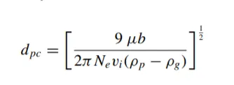
where N_e is the number of revolutions     

                                          

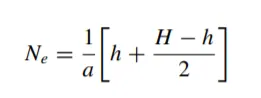
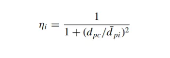
The efficiency of collection of any size of particle is given by

                                 

Simulation:

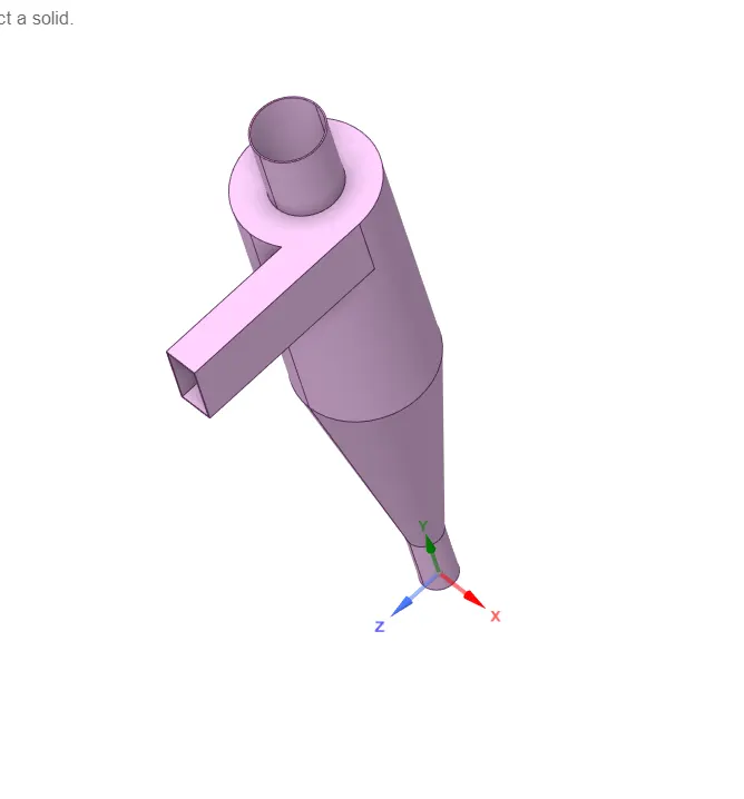
1. import the model in space claim and extract volume and delete other parts.
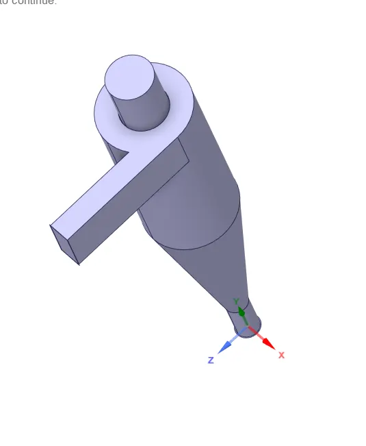
2. open the model in mesh and generate mesh with cartesian method.(*it is because there we several minute geomentries which makes impossible for normal mesh to create)
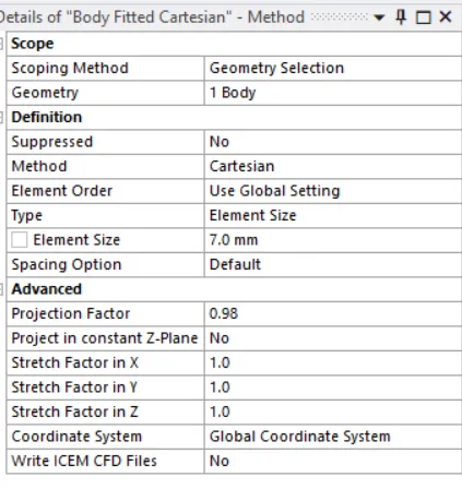
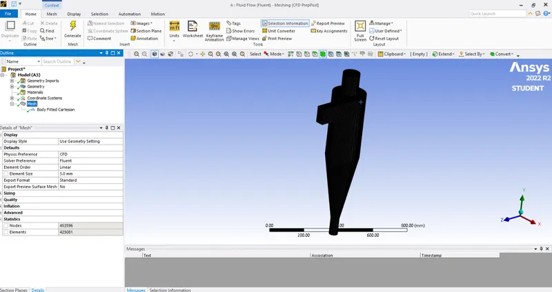
3. set mesh size for 5mm size
4. open fluent and set gravity as 9.81m/s2
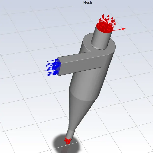
5. steady state solver>>viscous model >> k-epsilon>>rng>> swirl dominant flow
6. discrete phase model>>interact with continous phase>>update dpm sources every flow interaction>>injections >> create>> material >> anthracite >>surface injection type >> size: 1 e-6 mm and velocity 3 m/s
7. set boundary condition as inlet velocity 3m/s and dpm reflect>>outlet top>>dpm escape>> outlet bottom>> dpm trap>>wall >> dpm reflect
8. initialize simulation and run for 1000 iterations plot pr drop at inlet
9. after simulation export particle data file 
10. open cfd and import saved particle data file and view particle time seperator
11. follow the same different particle size as 3 and 5micro meter and also vary velocity for 1 and 5m/s
12. compare obtained results
13. for calculating efficiency 

seperator efficiency= trapped particles/tracked particles

observation:

Case 1:

at velocity 3m/s

s.no	particle size	residuals	pr drop at inlet	pr drop	particle tracking	efficiency
1	1 micro meter		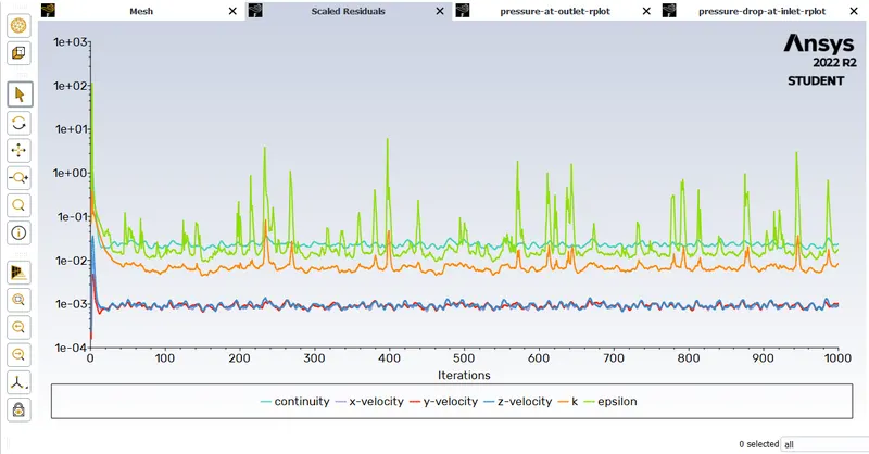	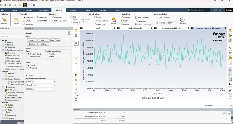7.8pa		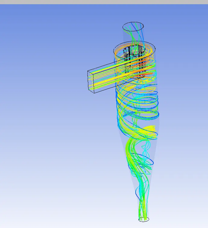n=(275/378) n=72.7%
2	3 micro meter		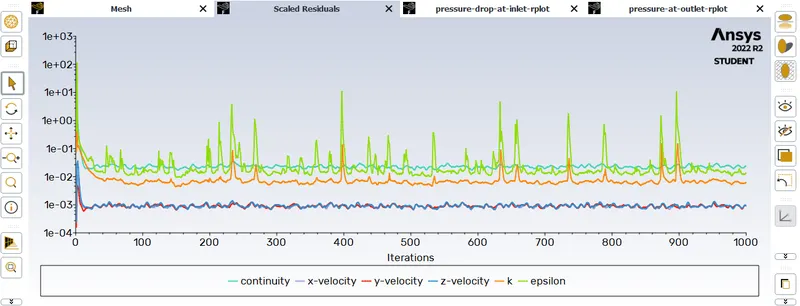	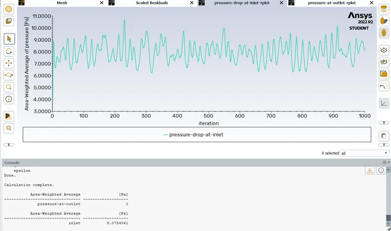8.07pa		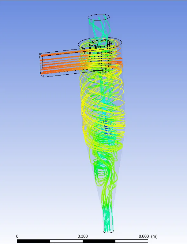n= 240/378 n=63.4%
3	5 micrometer		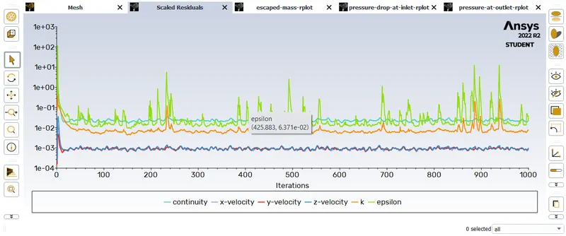	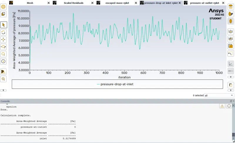8.31pa		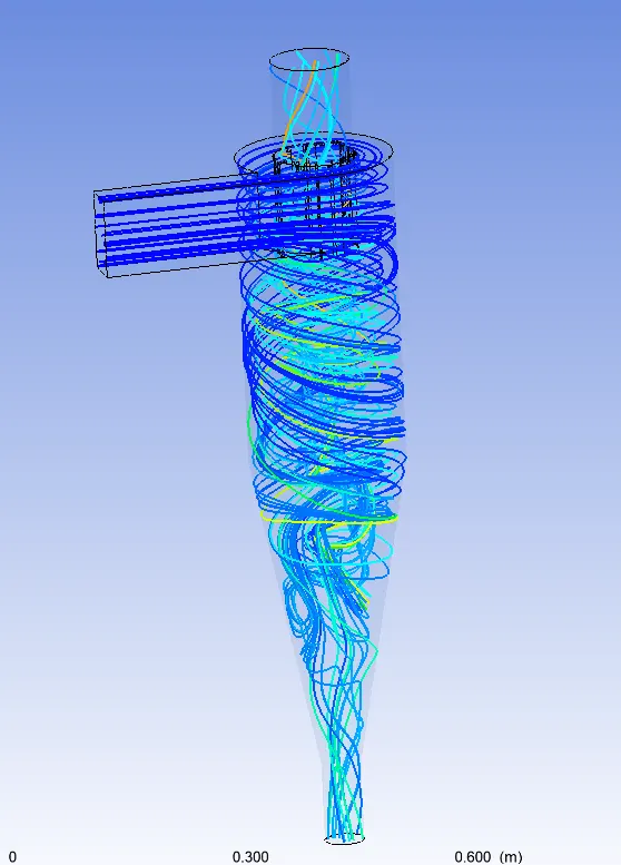n=202/378 n=53.4%

 case 2:

size 5 micrometer

s.no	velocity	residuals	pr drop plot	pr drop at inlet	particle tracking	efficiency
1	1m/s		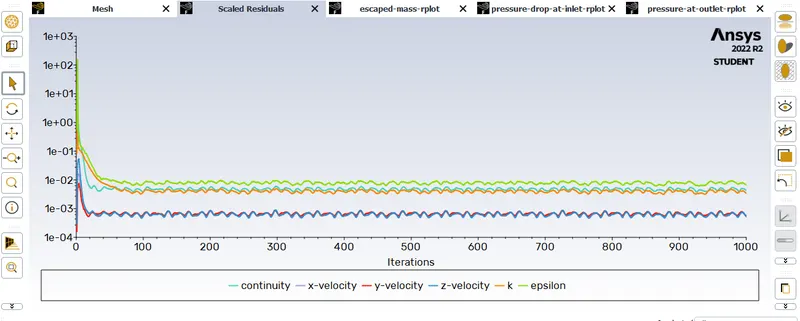	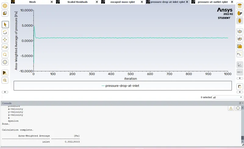8.07 pa		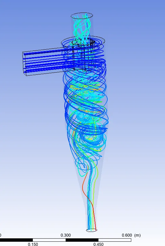n= 131/378 n=34.6%
2	3 m/s			8.31pa		n=202/378 n=53.4%
3	5m/s		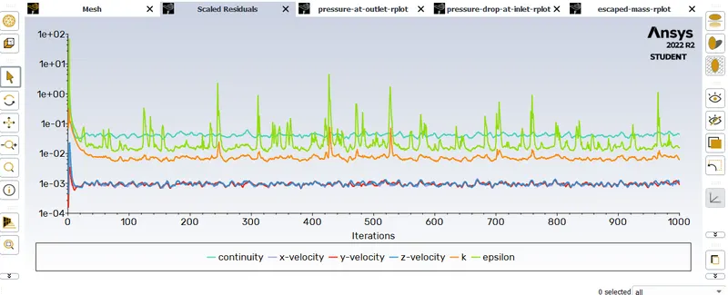	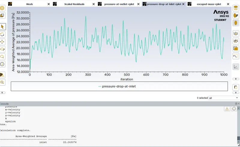8.8pa		n=275/378 n= 72.7%

Results:

while comparing the case 1 results it can be shown clearly that size of the particle is indirectly proportional to efficiency . it states that lower the particle size higher the efficiency.

while observing the case 2 results it can be shown that increase in velocity will results in increased efficiency.