Week 8 - Simulating Cyclone separator with Discrete Phase Modelling
Aim:- To perform analysis on cyclone separator and calculate the separation efficiency and pressure drop.
Objective:-
- To write a few words about any four empirical models used to calculate the cyclone separator efficiency.
- To perform an analysis on a given cyclone separator model by varying the particle diameter from 1 μm to 5 μm and calculate the separation efficiency in each case. Discuss the results. [Use both the velocity's as 3m/sec.]
- To perform an analysis on a given cyclone separator model by varying the particle velocity from 1 m/sec to 5 m/sec and calculate the separation efficiency and pressure drop in each case. Discuss the results. [Use particle diameter size as 5 μm for all cases & keep flow velocity same as particle velocity]
Introduction:
Cyclonic separation is a method of removing particulates from an air, gas or liquid stream, without the use of filters, through vortex separation. When removing particulate matter from liquid, a hydrocyclone is used; while from gas, a gas cyclone is used. Rotational effects and gravity are used to separate mixtures of solids and fluids. The method can also be used to separate fine droplets of liquid from a gaseous stream.
A high speed rotating (air)flow is established within a cylindrical or conical container called a cyclone. Air flows in a helical pattern, beginning at the top (wide end) of the cyclone and ending at the bottom (narrow) end before exiting the cyclone in a straight stream through the center of the cyclone and out the top. Larger (denser) particles in the rotating stream have too much inertia to follow the tight curve of the stream, and thus strike the outside wall, then fall to the bottom of the cyclone where they can be removed. In a conical system, as the rotating flow moves towards the narrow end of the cyclone, the rotational radius of the stream is reduced, thus separating smaller and smaller particles. The cyclone geometry, together with volumetric flow rate, defines the cut point of the cyclone. This is the size of particle that will be removed from the stream with a 50% efficiency. Particles larger than the cut point will be removed with a greater efficiency, and smaller particles with a lower efficiency as they separate with more difficulty or can be subject to re-entrainment when the air vortex reverses direction to move in direction of the outlet.
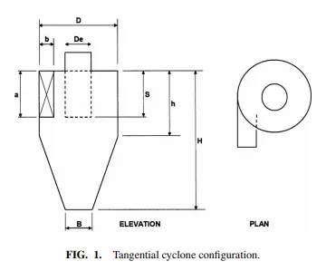
Large scale cyclones are used in sawmills to remove sawdust from extracted air. Cyclones are also used in oil refineries to separate oils and gases, and in the cement industry as components of kiln preheaters. Cyclones are increasingly used in the household, as the core technology in bagless types of portable vacuum cleaners and central vacuum cleaners. Cyclones are also used in industrial and professional kitchen ventilation for separating the grease from the exhaust air in extraction hoods.[2] Smaller cyclones are used to separate airborne particles for analysis. Some are small enough to be worn clipped to clothing, and are used to separate respirable particles for later analysis
empirical models used to calculate the cyclone separator efficiency.
IOZIA AND LEITH MODEL
The model assumes that a particle carried by the vortex endures the influence of two forces: a centrifugal force, Z, and a flow resistance, W. Core length, zc, and core diameter,
dc, are given as
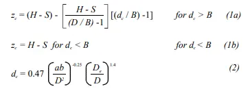
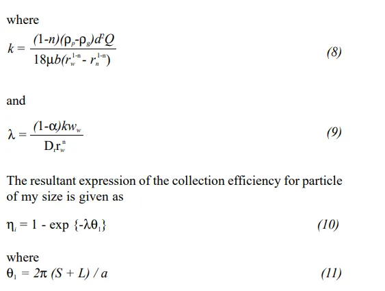
The addition made by Iozia and Leith on the original Barth(1956) model are the core length zc and slope parameter β expression which is derived based on the statistical analysis of experimental data of cyclone with D = 0.25 m. The collection efficiency ηi of particle diameter dpi can be calculated from
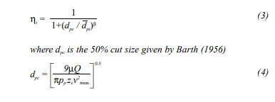
2 LI AND WANG MODEL
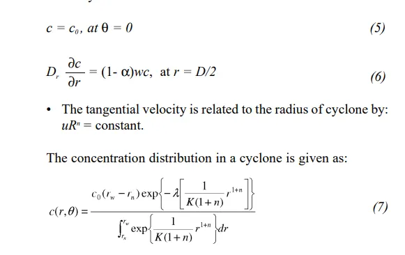
The Li and Wang (1989) model includes particle bounce or re-entrainment and turbulent diffusion at the cyclone wall. A two-dimensional analytical expression of particle distribution in the cyclone is obtained. Li and Wang model was developed based on the following assumptions:
• The radial particle velocity and the radial concentration profile are not constant, for uncollected particles within the cyclones.
• Boundary conditions with the consideration of turbulent diffusion coefficient and particle bounce re-entrainment on the cyclone wall are:
• The tangential velocity is related to the radius of cyclone by: uRn = constant.
The concentration distribution in a cyclone is given as:
KOCH AND LICHT MODEL
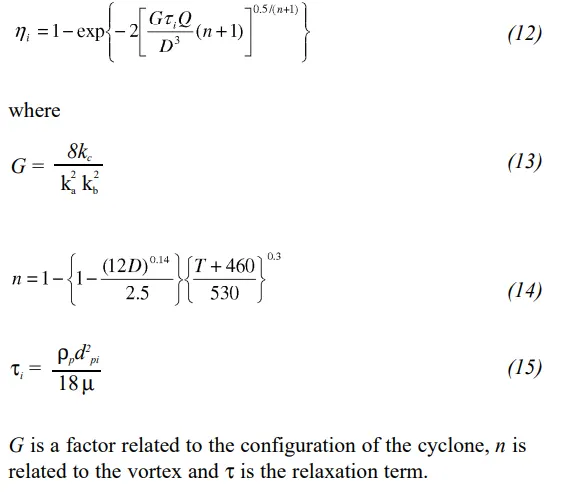
Koch and Licht (1977) collection theory recognized the inherently turbulent nature of cyclones and the distribution of gas residence times within the cyclone. Koch and Licht describe particle motion in the entry and collection regions with the additional following assumptions:
• The tangential velocity of a particle is equal to the tangential velocity of the gas flow, i.e. there is no slip in the tangential direction between the particle and the gas.
• The tangential velocity is related to the radius of cyclone by:
uRn = constant.
A force balance and an equation on the particles collection
yields the grade efficiency ηi
LAPPLE MODEL
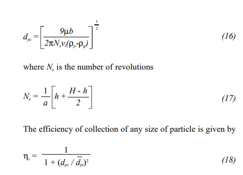
Lapple (1951) model was developed based on force balance without considering the flow resistance. Lapple assumed that a particle entering the cyclone is evenly distributed across the inlet opening. The particle that travels from inlet half width to the wall in the cyclone is collected with 50% efficiency. The semi empirical relationship developed by Lapple (1951) to calculate a 50% cut diameter, dpc, is
Procedure:
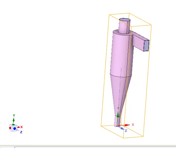
step 1: import the geometry into space claim and extract the fluid volume.
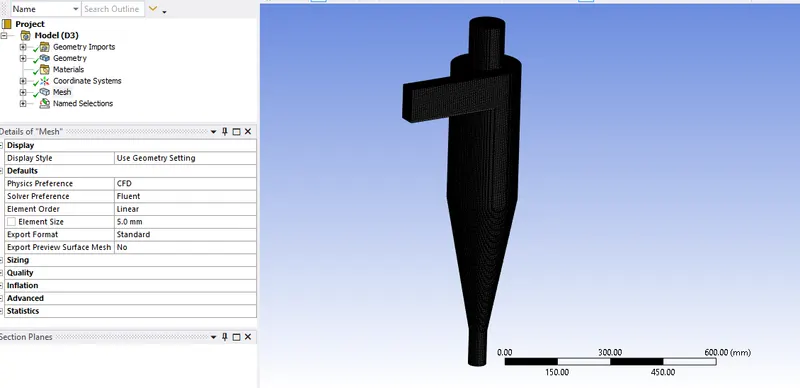
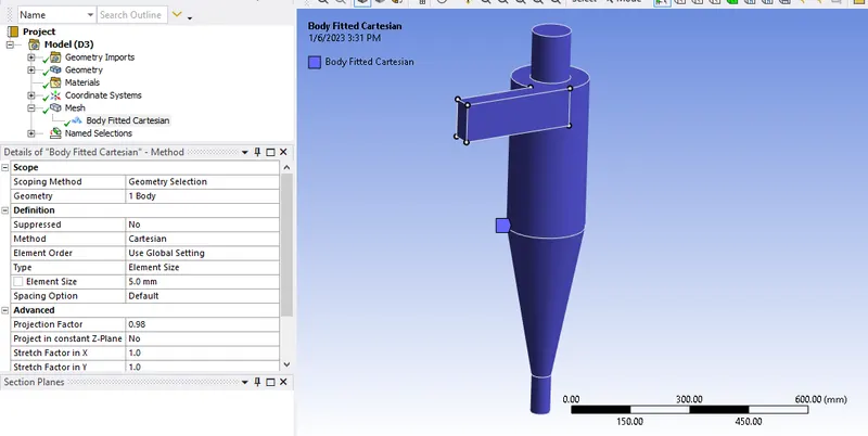
step 2: create a mesh setup
1. element size: 5mm
2. Method = Cartesian method
3. Cartesian element size= 5 mm
no of elements= 427871
step 3: create a name selection for the respective faces as inlet outlet surfaces
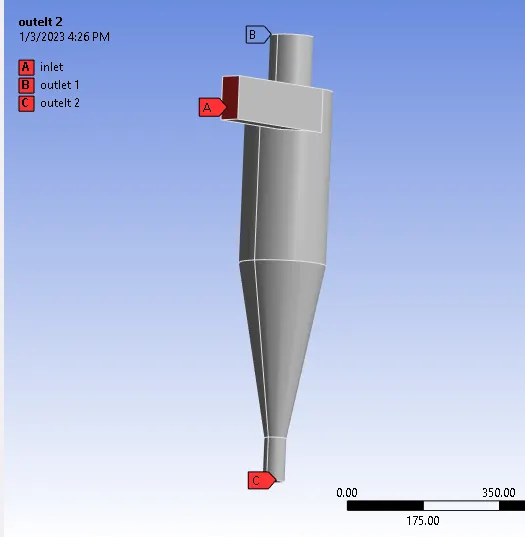
step 4: open fluent setup, follow below procedure for all the cases which involves varying the particle diameter and velocities as per requirement.
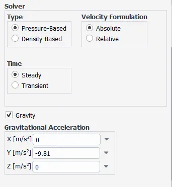
- under general->click on Pressure based solver-> Steady state analysis ->absolute velocity->gravity is enabled where acceleration due to gravity = 9,81 m/s in negative direction is inputted.
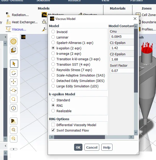
- under viscous->use k-epsilon model RNG->swirl dominated flow.
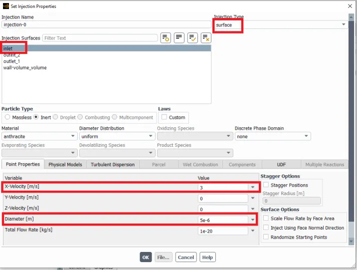
- In this particular model we are using discreet phase modelling to perform the simulation, so click on the discreet under physics and enable marked phase as shown in the below snap and click on injection and input the velocity=3m/s and diameter=5e-06m, For injection, the particle type is inert. From fluent database , anthracite is selected. It is released from the inlet,
note: velocity and diameter of antracite particle diameter values are changed for different cases.
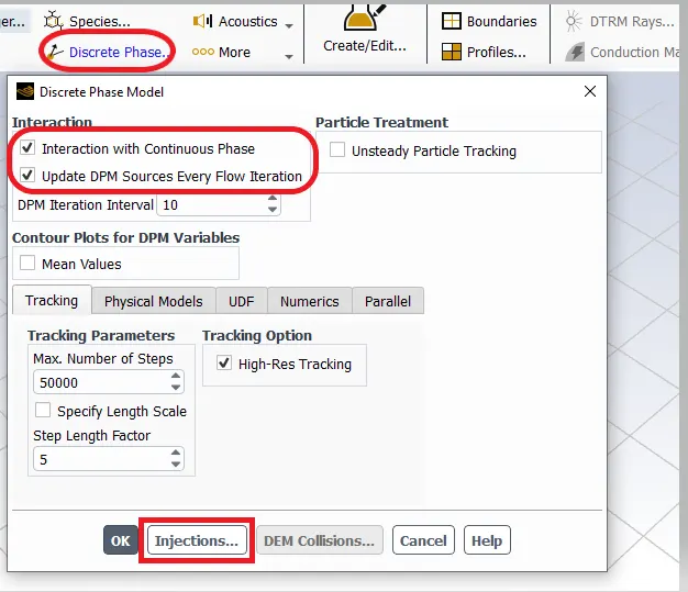
here we will understand the meaning of discreet phase modeling.
The discrete Phase Model is a subsection of Multiphase flows. A discrete phase model (DPM) is used when the aim is to investigate the behavior of the particles from a Lagrangian view and a discrete perspective. The difference between the Lagrangian and the Eulerian view is that fluid behavior in the Lagrangian view is examined based on particle tracking of a particulate flow, whereas fluid behavior is considered in the Eulerian view based on the assumption of a finite volume element in the fluid flow path.
In Discrete Phase Model, the continuous phase is solved using Navier-Stokes equations. At the same time, the discrete phase is simulated by tracking a large number of particles, bubbles, or droplets passing through the calculated continuous flow field. It should be noted that the discrete phase can exchange momentum, mass, and energy with the continuous phase. This method can be made much simpler by ignoring the interaction of particles (as well as droplets and bubbles) with each other. Of course, this can happen when the discrete phase, even with a large mass, has a much smaller volume (less than 10%) than the continuous phase. After each iteration of the continuous phase calculations, the particle paths are calculated and determined separately.
The Discrete Phase in ANSYS FLUENT can be used to model different types of phenomena, including:
- calculation of the discrete phase trajectory using a Lagrangian formulation that includes the discrete phase inertia, hydrodynamic drag, and the force of gravity for both steady and unsteady flows
- prediction of the effects of turbulence on the dispersion of particles due to turbulent eddies present in the continuous phase
- heating/cooling of the discrete phase
- vaporization and boiling of liquid droplets
- combusting particles, including volatile evolution and char combustion to simulate coal combustion
- droplet breakup and coalescence
- Erosion or accretion
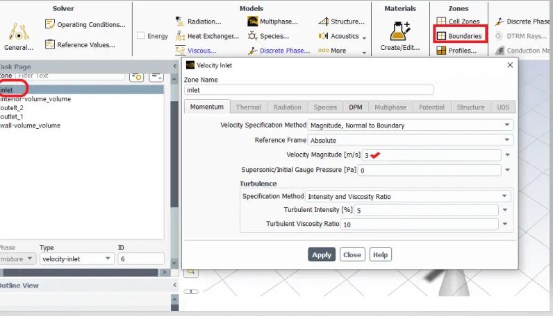
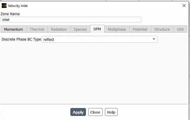
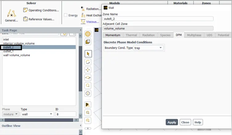
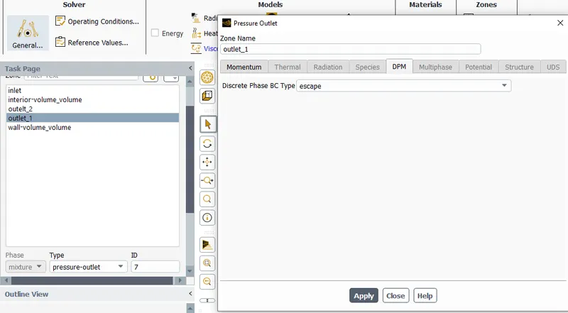
- under boundary input the conditions and values and required DPM BC type as below.
inlet and wall:- Reflect
Outlet(Top):- Escape
Outlet(Bottom/dustbin) - Trap
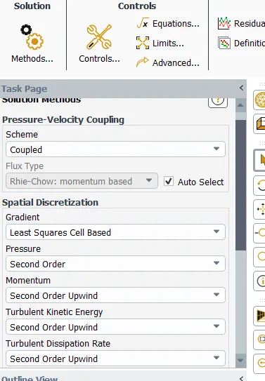
- Solution methods:
-
COUPLED scheme is chosen . The gradient being least square cells based. Pressure,Momentum, Turbukent kinetic energy and turbulent dissipation rate is second order upwind in order to reduce the computational time.
- The solution is initialized using standard intialization and under options it is computed from inlet region
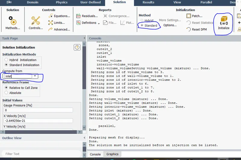
- the analysis is carried out for 600 iterations and residuals are plotted.
- The particle solution data is exported under file->export->particle data->click on injection 0-> select the path and import the data file in CFD post.
Results:
case 1
1) particle diameter=1μm,velocity=3m/s
number tracked = 378, escaped = 67, trapped = 311
separation efficiency =(number of particles trapped/number of particles tracked )*100
= (311/378)*100
= 82.27%
pressure drop=Total inlet pressure-Total outlet pressure
=23.0947-(-0.0075)
=23.1022Pa
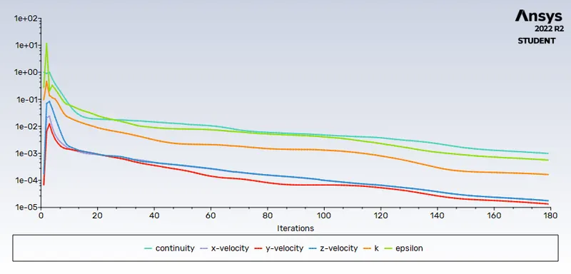
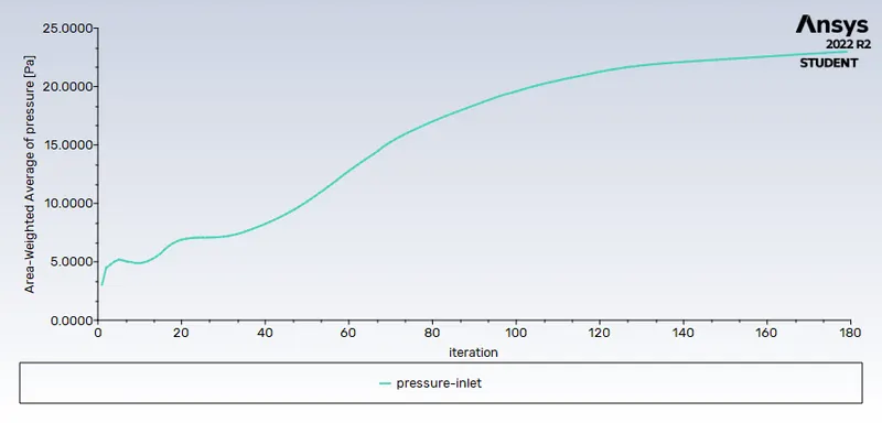
Residuals pressure inlet= 23.0947 Pa
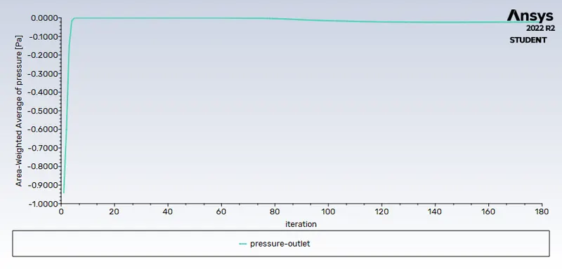
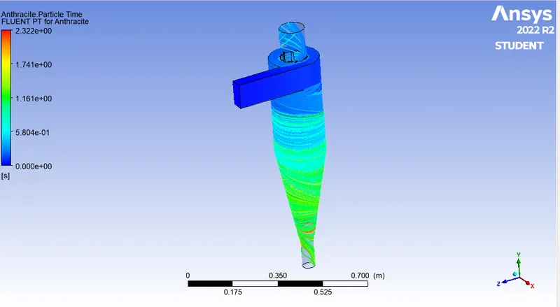
pressure-outlet=-0.0075Pa Particle time
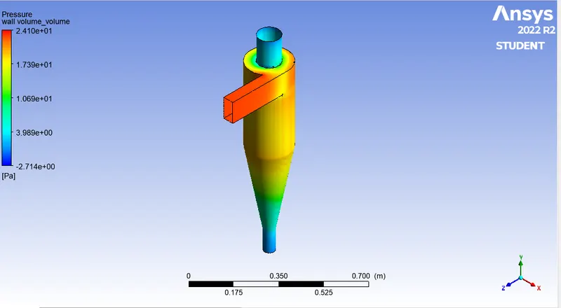
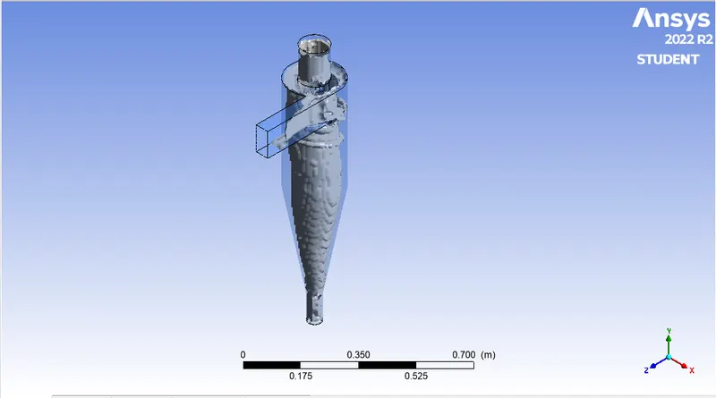
pressure contour swril strength at 0.002
2) particle diameter=3μm,velocity=3m/s
number tracked = 378, escaped = 62, trapped = 316
separation efficiency =(number of particles trapped/number of particles tracked )*100
= (316/378)*100
= 83.59%
pressure drop=Total inlet pressure-Total outlet pressure
=23.0947-(-0.0075)
=23.1022Pa
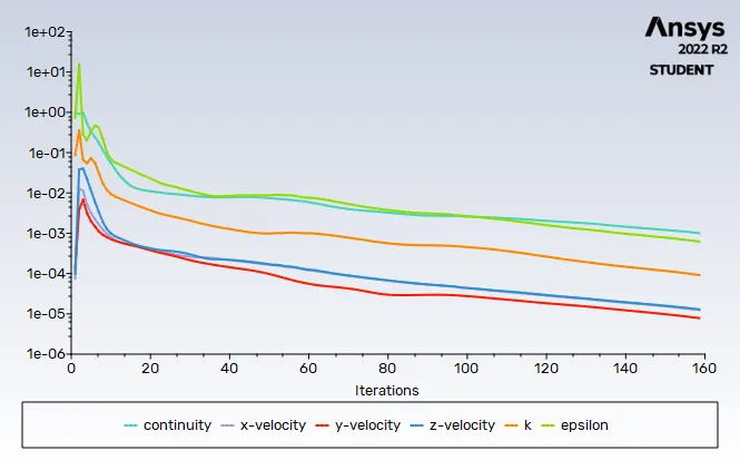
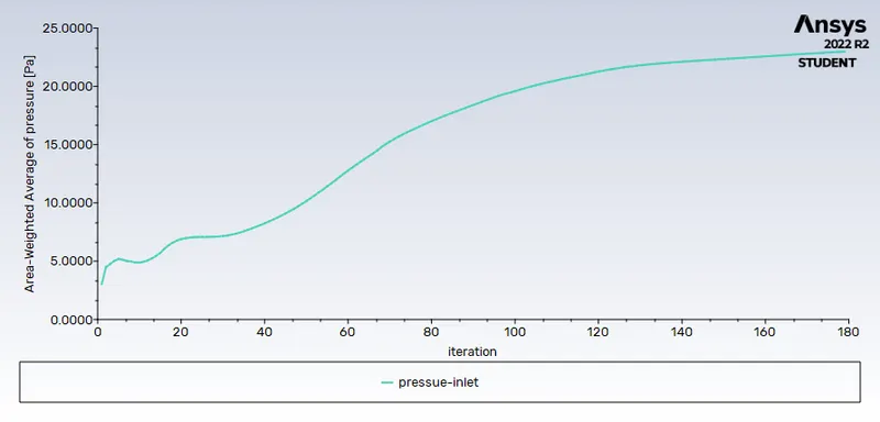
Residuals pressure inlet= 23.0947 Pa
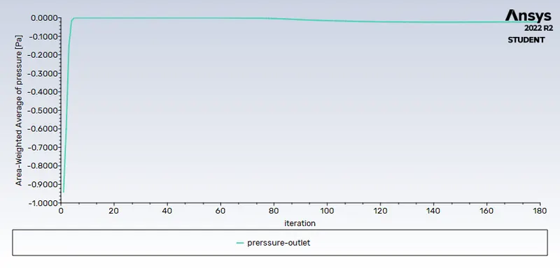
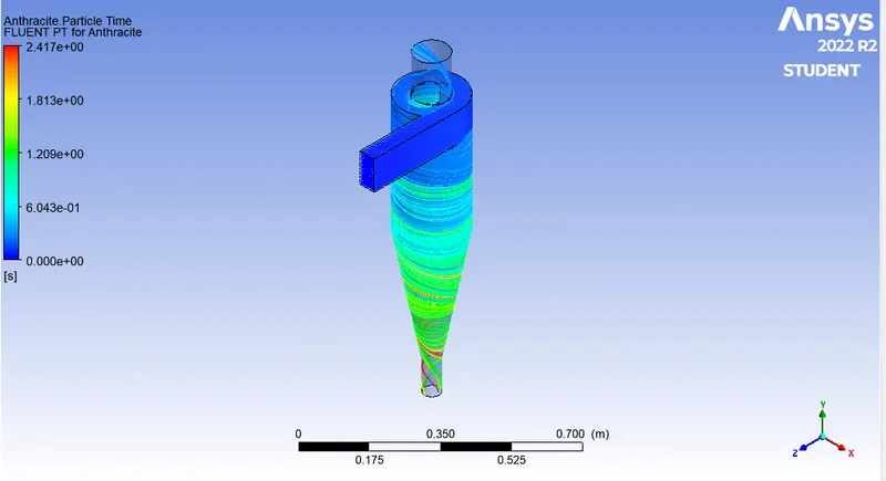
pressure-outlet=-0.0075Pa Particle time
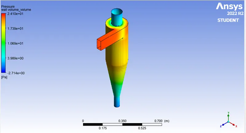
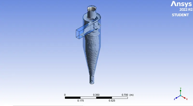
pressure contour swril strength at 0.002
3)particle diameter=5μm,velocity=3m/s
number tracked = 378, escaped = 92, trapped = 286
separation efficiency =(number of particles trapped/number of particles tracked )*100
= (286/378)*100
= 75.66%
pressure drop=Total inlet pressure-Total outlet pressure
=23.0947-(-0.0075)
=23.1022Pa
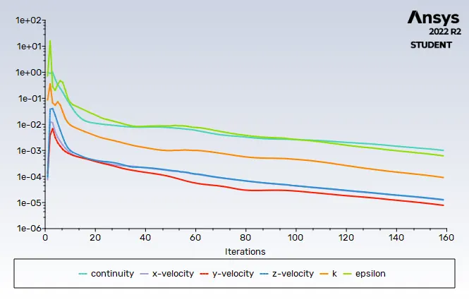
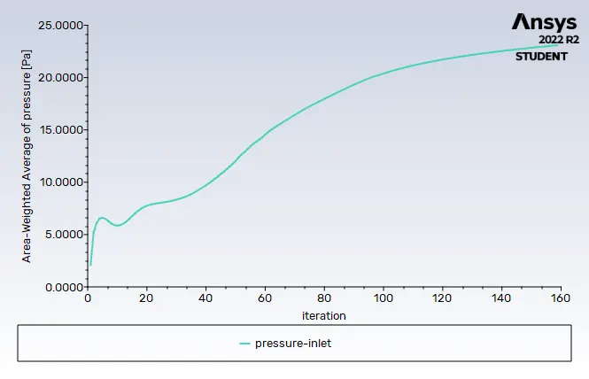
Residuals pressure inlet= 23.0947 Pa
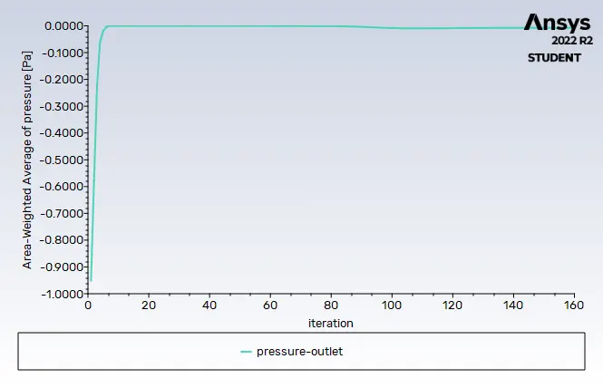
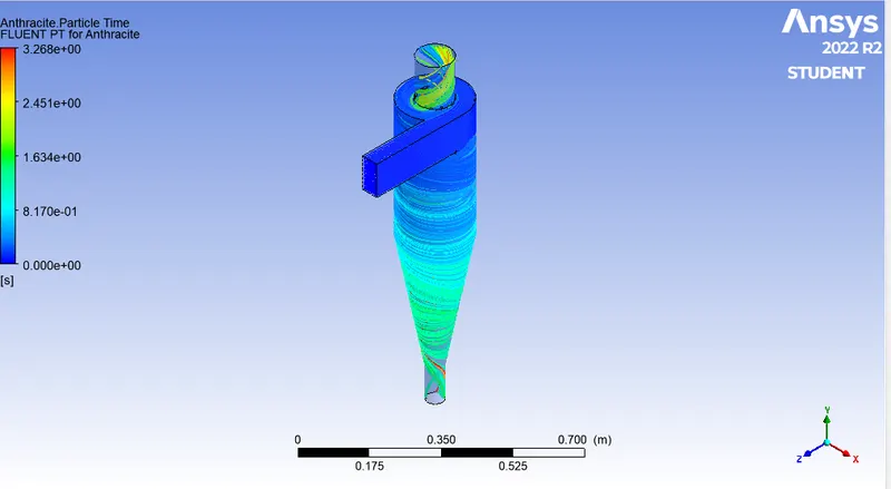
pressure-outlet=-0.0075Pa Particle time
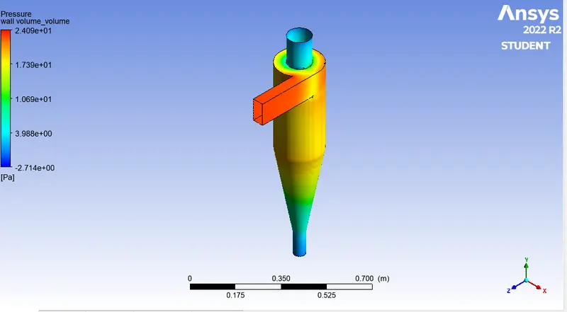
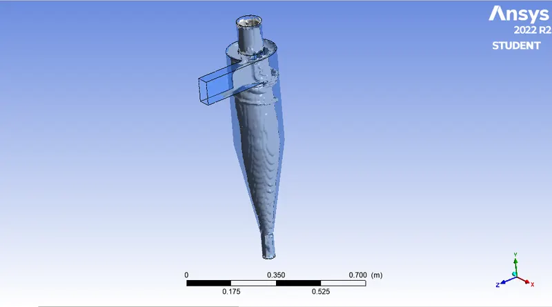
pressure contour swril strength at 0.002
Case 2
1)particle diameter=5μm,velocity=1m/s
number tracked = 378, escaped = 71, trapped = 307
separation efficiency =(number of particles trapped/number of particles tracked )*100
= (307/378)*100
= 81.21%
pressure drop=Total inlet pressure-Total outlet pressure
=1.9063-(-1.1829)
=3.0892Pa
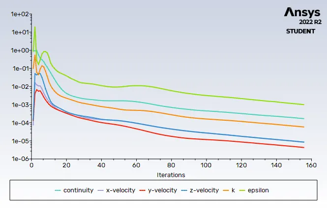
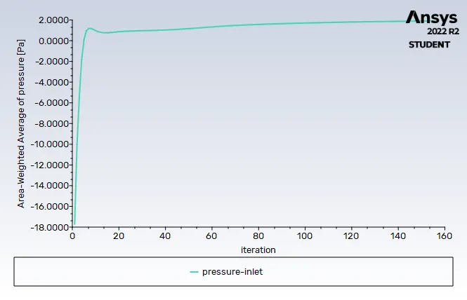
Residuals pressure inlet=1.9063Pa
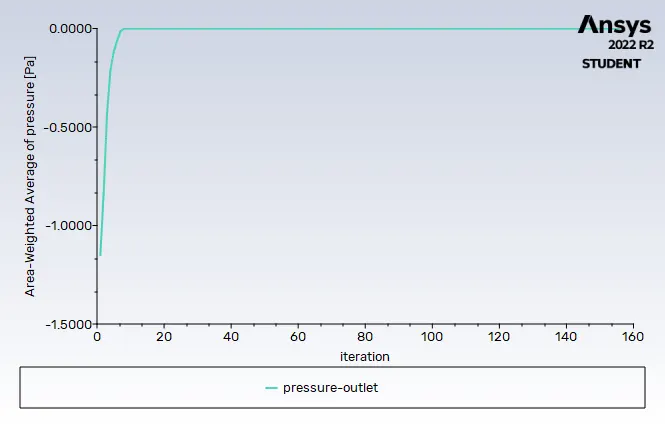
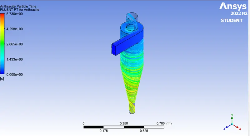
pressure-outlet=1.1829Pa Particle time
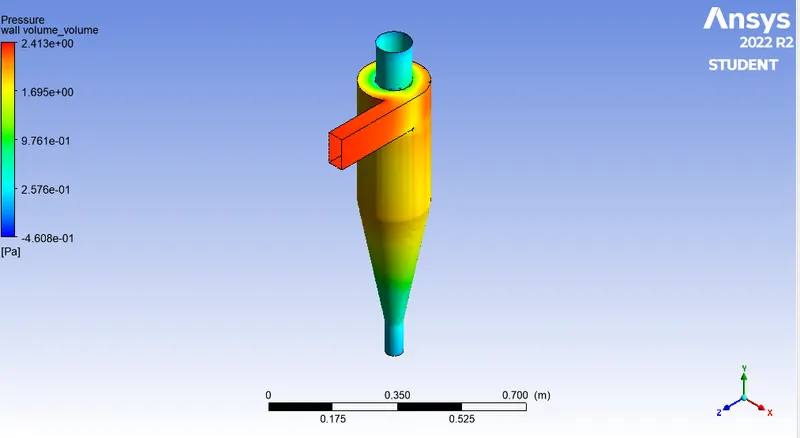
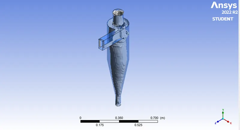
pressure contour swril strength at 0.002
1)particle diameter=5μm,velocity=5m/s
number tracked = 378, escaped = 90, trapped = 288
separation efficiency =(number of particles trapped/number of particles tracked )*100
= (288/378)*100
= 76.19%
pressure drop=Total inlet pressure-Total outlet pressure
=23.0947-(-0.0075)
=23.1022Pa
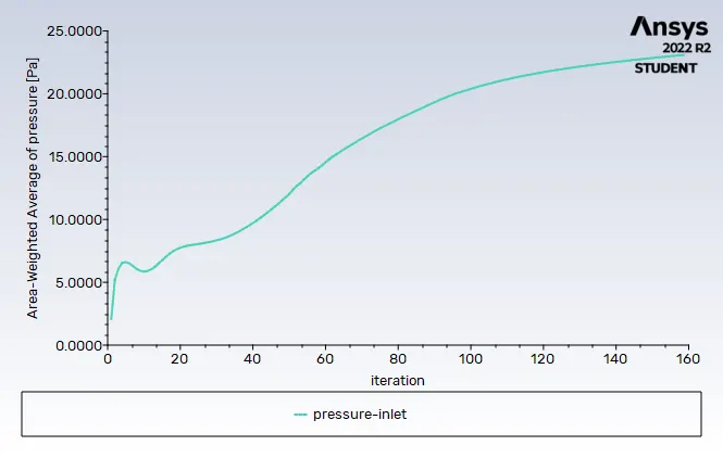
Residuals pressure inlet=23.0947Pa
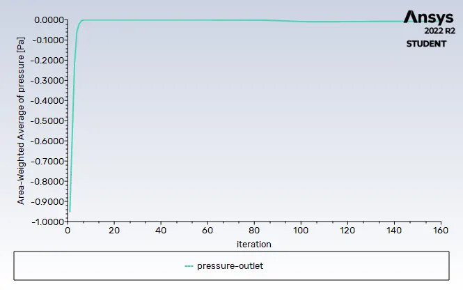
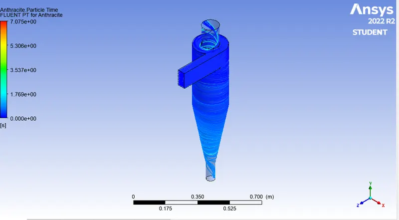
pressure-outlet=-0.0075Pa Particle time
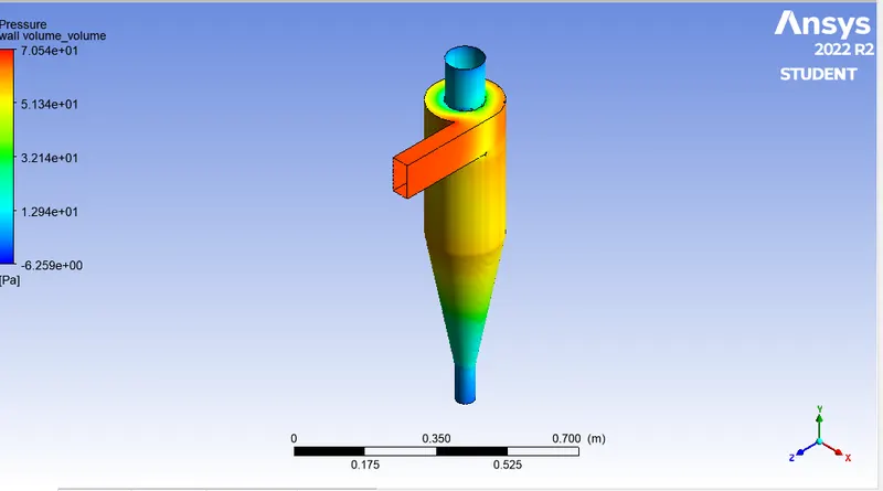
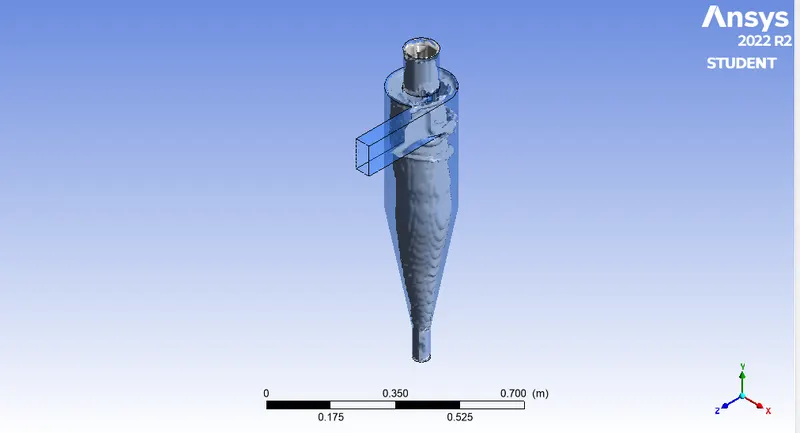
pressure contour swril strength at 0.002
Final results tabulation:
| Cases |
Particle diameter (μm) |
velocity (m/s) |
separation efficiency (%) |
Pressure drop (Pa) |
| 1 | 1 | 3 | 82.27 | 23.1022 |
| 1 | 3 | 3 | 83.59 | 23.1022 |
| 1 & 2 | 5 | 3 | 75.66 | 23.1022 |
| 2 | 5 | 1 | 81.21 | 3.0892 |
| 2 | 5 | 5 | 76.19 | 23.1022 |
Conclusion:
- To reduce the computational effort, the RNG k-epsilon model was be used with enhancements wall treatment, RNG k-epsilon model underestimates the variation of the axial velocity profile across the radial direction and also overestimates the magnitude of the tangential velocity and the cyclone pressure drop
- The finite volume method has been used to discretize the partial differential equations of the model using the COUPLED method for pressure-velocity coupling and the Second Order
Upwind scheme to interpolate the variables on the surface of the control volume. - From the above results we can conclude that as the velocity increases the separation efficiency decreases, and this can be optimized by altering the dimensions of the cyclone separator and we otained pressure drop and we can see that it is same almost all the cases.