Week 8 - Simulating Cyclone separator with Discrete Phase Modelling
In this project, a cyclone separator will be simulated using ANSYS Fluent and Discrete Phase Modelling.
A cyclone separator uses inertia to remove impurities or small particles from flowing fluid. They are used as pollution control devices to reduce the amount of polluntant particles from entering the atmosphere. It is preferred due to its lack of moving parts, but it cannot effectively filter out smaller particles.
A discrete phase model (DPM) is used when the aim is to investigate the behavior of the particles from a Lagrangian view and a discrete perspective. A DPM is a part of the Multiphase model seen in other instances such as gearboxes or Rayleigh-Taylor instability. The difference between the Lagrangian and the Eulerian view is that fluid behavior in the Lagrangian view is examined based on particle tracking of a particulate flow; Whereas fluid behavior is considered in the Eulerian view based on the assumption of a finite volume element in the fluid flow path.
Separation Efficiency
Seperation Efficiency is defined as the ratio of the concentration of particles removed from the incoming flow to the concentration of particles in the incoming stream.
Mathematically,
`eta_(separation) = ((M_(cl ean air))/(M_(mixtureair)))xx100%`
For this project,
`eta_(separation) = ((M_(outl et1))/(M_(i nl et)))xx100%`
where `M_(outl et1)` is the mass flow rate at the outlet and `M_(i nl et)` is the mass flow rate at the inlet.
There are 4 methods used to calculate separation efficiency, they are
1. The Li and Wang (1989) model includes particle bounce or re-entrainment and turbulent dif fusion at the cyclone wall. A two-dimensional analytical expression of particle distribution in the cyclone is obtained.
2. Iozia and Leith (1990) logistic model is a modified version of Barth (1956) model which is developed based on force balance. The model assumes that a particle carried by the vortex endures the influence of two forces: a centrifugal force and a flow resistance.
3. Koch and Licht (1977) collection theory recognized the inherently turbulent nature of cyclones and the distribution of gas residence times within the cyclone. Koch and Licht describe particle motion in the entry and collection regions
with the additional following assumptions:
• The tangential velocity of a particle is equal to the tangential
velocity of the gas flow, i.e. there is no slip in the tangential
direction between the particle and the gas.
• The tangential velocity is related to the radius of cyclone
4. Lapple (1951) model was developed based on force balance without considering the flow resistance. Lapple assumed that a particle entering the cyclone is evenly distributed across the inlet opening. The particle that travels from inlet half width to the wall in the cyclone is collected with 50% efficiency.
This project will mainly focus on the effects of changing the particle size and inlet velocity on the separation efficiency and pressure drop across the separator.
The simulation will be conducted for 4 cases, they are:
1. Inlet velocity: `3m//s`, particle size: `1 mum`
2. Inlet velocity: `5m//s`, particle size: `1 mum`
3. Inlet velocity: `1m//s`, particle size: `5 mum`
4. Inlet velocity: `5m//s`, particle size: `5 mum`
Geometry
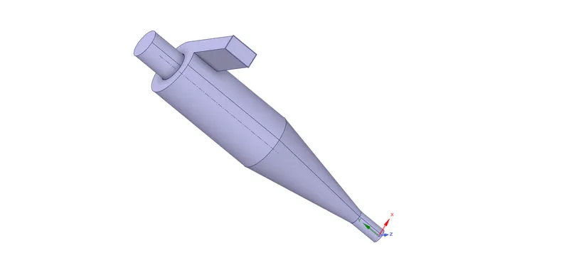
The geometry is imported as a .STEP file into SpaceClaim. The imported geometry's volume is extracted, as the simulation is about a fluid flowing in the volume. The separator is supressed, this is the final geometry:
Meshing
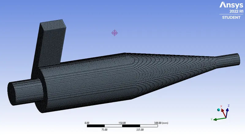
The base mesh size is 10 mm. An additional control was introduced to ensure a patch conforming mesh with the boundary is generated.
Controls -> Method -> Cartesian
This is the resulting mesh:
Zooming in,
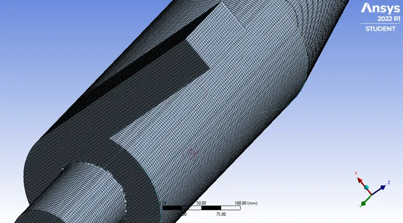
This mesh contains 453596 nodes and 425081 elements.
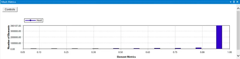
From the mesh metrics, most elements have a quality >0.9, this indicates the mesh quality is satisfactory.
Simulation Setup
Solver - General
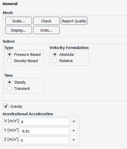
This simulation ran on a steady state, 3D and with gravity enabled.
Turbulence Model
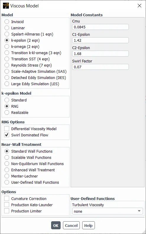
keps was the preffered turbulence model due to its excellence in handling swirls.
Discrete Phase Modelling
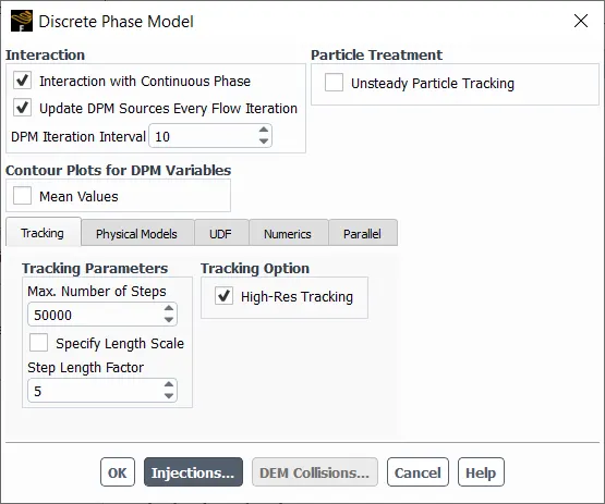
In this stage, the heavier particles are added to the simulation.
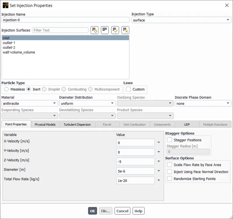
The heavier particle in this project is anthracite, a type of coal. The particles are defined to enter the domain at the inlet, normal to the inlet at a velocity equal to the flow velocity. The finer the mesh, the more number of particles introduced.
Boundaries
inlet: velocity inlet with reflect DPM condition
outlet-1: pressure outlet with escape DPM condition (upper outlet, clean air)
outlet-2: pressure outlet with trap DPM condition (lower outlet, particulate rich air)
wall: wall with reflect DPM condition
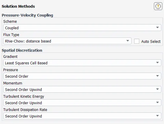
Solution Methods
Turbulent K.E. and Turbulence D.R. were changed to Second Order Upwind.
Simulation Results
The simulation was ran with the same setup for all four cases and the results are below:
Case 1
The inlet velocity is`3m//s` and the particle size is`1 mum`. The simulation was ran until it reached a steady state.
Residuals
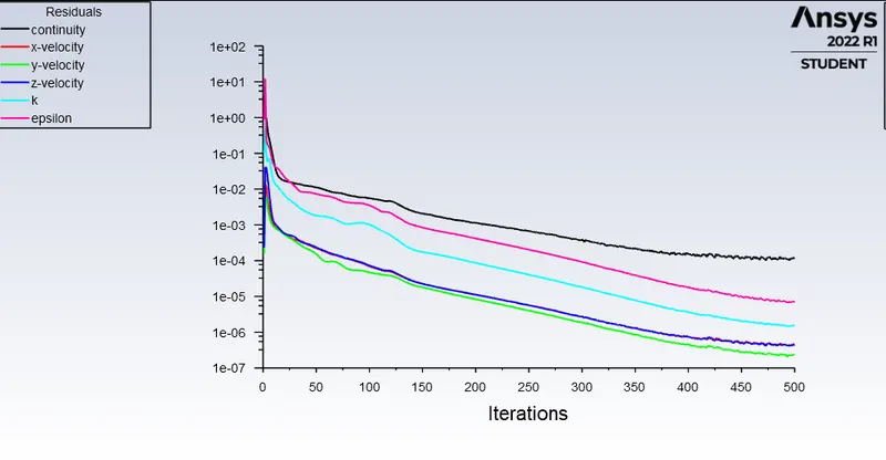
The simulation took 500 iterations. The solution is said to be converged as the residuals are low and cannot go any lower.
Animation
Taken in CFD-Post
Separation Efficiency Calculation
Mass flow values were taken using the function calculator in CFD-Post.
Mass flow rate at inlet: 0.0183815 `kg//s`
Mass flow rate at outlet 1: -0.0152712 `kg//s`
Mass flow rate at outlet 2: -0.00306893 `kg//s`
Note: mass flow rate is negative at the outlets because mass is leaving the domain. Hence, the negative sign is ignored in all calculations.
`eta_(separation) = ((M_(outl et1))/(M_(i nl et)))xx100%`
`eta_(separation) = (0.0152712/0.0183815)xx100%`
`eta_(separation) = 83.079%`
Case 2
The inlet velocity is`5m//s` and the particle size is`1 mum`. The simulation was ran until it reached a steady state.
Residuals
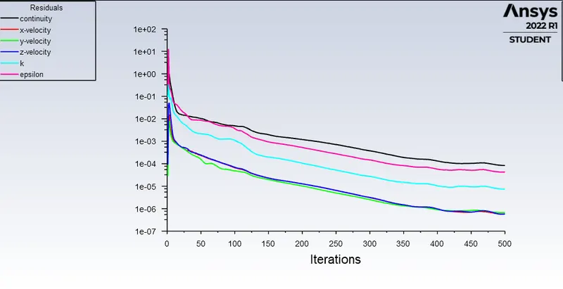
The simulation took 500 iterations. The solution is said to be converged as the residuals are low and cannot go any lower.
Animation
This was taken in CFD-Post
Separation Efficiency Calculation
Mass flow values were taken using the function calculator in CFD-Post.
Mass flow rate at inlet: 0.0306359 `kg//s`
Mass flow rate at outlet 1: -0.0254254`kg//s`
Mass flow rate at outlet 2: -0.00513781`kg//s`
Note: mass flow rate is negative at the outlets because mass is leaving the domain. Hence, the negative sign is ignored in all calculations.
`eta_(separation) = ((M_(outl et1))/(M_(i nl et)))xx100%`
`eta_(separation) = (0.0254254/0.0306359)xx100%`
`eta_(separation) = 82.99%`
Case 3
The inlet velocity is`1m//s` and the particle size is`5 mum`. The simulation was ran until it reached a steady state.
Residuals
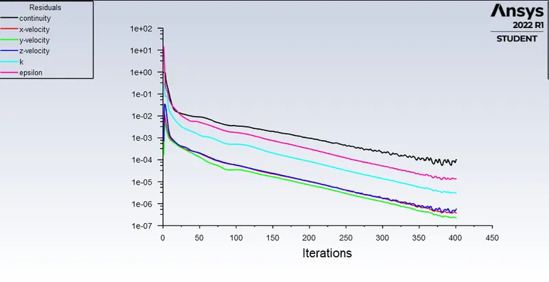
The simulation took 400 iterations. The solution is said to be converged as the residuals are low and have started to oscillate.
The maximum pressure is 2.235 Pa and the minimum pressure is -0.625 Pa. Hence, the pressure drop is 2.86 Pa.
Animation
This was taken in CFD-Post
Separation Efficiency Calculation
Mass flow values were taken using the function calculator in CFD-Post.
Mass flow rate at inlet: 0.00612717`kg//s`
Mass flow rate at outlet 1: -0.00508355`kg//s`
Mass flow rate at outlet 2: -0.00103245`kg//s`
Note: mass flow rate is negative at the outlets because mass is leaving the domain. Hence, the negative sign is ignored in all calculations.
`eta_(separation) = ((M_(outl et1))/(M_(i nl et)))xx100%`
`eta_(separation) = (0.00508355/0.00612717)xx100%`
`eta_(separation) = 82.967%`
Case 4
The inlet velocity is`5m//s` and the particle size is`5 mum`. The simulation was ran until it reached a steady state.
Residuals
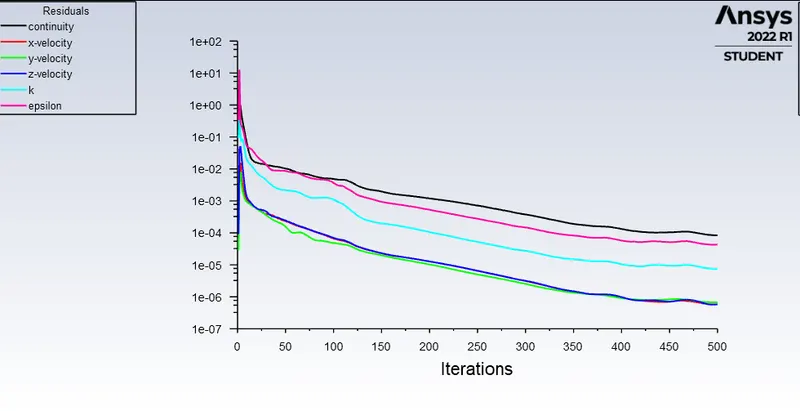
The simulation took 500 iterations. The solution is said to be converged as the residuals are low and cannot go any lower.
The maximum pressure is 78.075 Pa and the minimum pressure is -14.09 Pa. Hence, the pressure drop is 92.165 Pa.
Animation
This was taken in CFD-Post
Separation Efficiency Calculation
Mass flow values were taken using the function calculator in CFD-Post.
Mass flow rate at inlet: 0.0306359`kg//s`
Mass flow rate at outlet 1: -0.0254254`kg//s`
Mass flow rate at outlet 2: -0.00513781`kg//s`
Note: mass flow rate is negative at the outlets because mass is leaving the domain. Hence, the negative sign is ignored in all calculations.
`eta_(separation) = ((M_(outl et1))/(M_(i nl et)))xx100%`
`eta_(separation) = (0.0254254/0.0306359)xx100%`
`eta_(separation) = 82.992%`
Summary of Results
| Conditions | Separation Efficiency (`eta_(separation)`) |
| Inlet velocity: `3m//s`, particle size: `1 mum` | 83.079% |
| Inlet velocity: `5m//s`, particle size: `1 mum` | 82.995% |
| Inlet velocity: `1m//s`, particle size: `5 mum` | 82.967% |
| Inlet velocity: `5m//s`, particle size: `5 mum` | 82.992% |
Conclusions and Observations:
1. The simulation ran well and expected results were obtained.
2. The pressure drop calculated for case 3 and 4 is proportional to the inlet velocity.
3. The separation efficiency does not vary significantly with the inlet conditions, this can be perhaps explained that velocity was high when particle size was low.
4. It takes a lot of time for the heavier particles (relative to fluid particles) to circle down the separator, in this process the speed of the particles are reduced. This is a good thing as there is less chance of particles remixing with clean fluid.
5. The quick release of clean air is an advantage for cyclone separators, as a clean air supply is quick without any timelag.
References
1. B. Wang, D.L. Xu, K.W. Chu, A.B. Yu, Numerical study of gas–solid flow in a cyclone separator, Applied Mathematical Modelling, https://doi.org/10.1016/j.apm.2006.03.011.
2. Gimbun, Jolius & Luqman Chuah, Abdullah & Choong, TSY & Fakhru'l-Razi, A.. (2005). A CFD Study on the Prediction of Cyclone Collection Efficiency. International Journal for Computational Methods in Engineering Science and Mechanics. 6. 161-168. 10.1080/15502280590923649.