Week 3.5 - Deriving 4th order approximation of a 2nd order derivative using Taylor Table method

1. Central Difference

To calculate number of nodes for central differencing,

order of accuracy P = Number of nodes in the stencil N - order of derivative Q + 1

we know, P = 4, Q = 2. Solving for N we get N = 5

Let `(d^2f)/dx^2 = a f(i-2) + b f(i-1) + c f(i) + df(i+1) + e f(i+2)`

we have to create a taylor's table for the same

	`f(i)`	`Deltaxf'(i)`	`Deltax^2f''(i)`	`Deltax^3f'''(i)`	`Deltax^4f''''(i)`
`af(i-2)`	a	-2a	4a/2	-8a/6	16a/24
`bf(i-1)`	b	-b	b/2	-b/6	b/24
`cf(i)`	c	0	0	0	0
`df(i+1)`	d	d	d/2	d/6	d/24
`ef(i+2)`	e	2e	4e/2	8e/6	16e/24
	0	0	1	0	0

Adding the vertical columns we get,

`a+b+c+d+e=0`

`-2a-b+d+2e=0`

`2a+b/2+d/2+2e=1`

`-8a/6 - b/6 +d/6 +8e/6=0`

`16a/24 + b/24 + d/24 + 16e/24 = 0`

Simplyfying some equations and arranging them into matrix form, we get

`[[1,1,1,1,1],[-2,-1,0,1,2],[2,1/2,0,1/2,2],[-8,-1,0,1,8],[16,1,0,1,16]] [[a],[ b],[ c],[ d],[ e]] = [[0],[0],[1],[0],[0]]`

Solving this in MATLAB using the below code,

a=[1 1 1 1 1;-2 -1 0 1 2; 2 0.5 0 0.5 2;-4/3 -1/6 0 1/6 4/3; 2/3 1/24 0 1/24 2/3;]
b = [0 0 1 0 0]'
format rational
inv(a)*b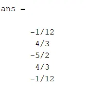

format rational was used to make sure the result is in p/q form else it may cause rounding errors later on

we get the resultant matrix which provides the solution or values of a, b, c, d and e

`a = -1/12`

`b=4/3`

`c=-5/2`

`d=4/3`

`e=-1/12`

Adding the 4th vertical column from Taylor's Table and we get: `f''(i)=(d^2f)/dx^2 = (a f(i-2) + b f(i-1) + c f(i) + df(i+1) + e f(i+2))/(Deltax^2)`

2. Right Skewed

To calculate number of nodes for right skewed differencing,

order of accuracy P = Number of nodes in the stencil N - order of derivative Q

we know, P = 4, Q = 2. Solving for N we get N = 6

Let `(d^2f)/(dx^2) = af(i) + bf(i+1) + cf(i+2)+df(i+3)+ef(i+4)+gf(i+5)`

now, a taylor's table for the same

	`f(i)`	`Deltaxf'(i)`	`Deltax^2f''(i)`	`Deltax^3f'''(i)`	`Deltax^4f''''(i)`	`Deltax^5f'''''(i)`
`af(i)`	a	0	0	0	0	0
`bf(i+1)`	b	b	b/2	b/6	b/24	b/120
`cf(i+2)`	c	2c	4c/2	8c/6	16c/24	32c/120
`df(i+3)`	d	3d	9d/2	27d/6	81d/24	243d/120
`ef(i+4)`	e	4e	16e/2	64e/6	256e/24	1024e/120
`gf(i+5)`	g	5g	25g/2	125g/6	625g/24	3125g/120
	0	0	1	0	0	0

Adding the vertical columns we get,

`a+b+c+d+e+g=0`

`b+2c+3d+4e+5g=0`

`b//2+4c//2+9d//2+16e//2+25g//2=1`

`b//6 + 8c//6+27d//6+64e//6+125g//6=0`

`b//24+16c//24+81d/24+256e//24+625g//24=0`

`b//120+32c//120+243d//120+1024e//120+3125g//120=0`

Simplyfying some equations and arranging them into matrix form, we get

`[[1,1,1,1,1,1],[0,1,2,3,4,5],[0,1,4,9,16,25],[0,1,8,27,64,125],[0,1,16,81,256,625],[0,1,32,243,1024,3125]][[a],[b],[c],[d],[e],[g]] = [[0],[0],[2],[0],[0],[0]]`

Solving this in MATLAB using the below code,

a=[1 1 1 1 1 1;0 1 2 3 4 5;0 1 4 9 16 25; 0 1 8 27 64 125; 0 1 16 81 256 625; 0 1 32 243 1024 3125;]
b = [0 0 2 0 0 0]'
format rational
inv(a)*b

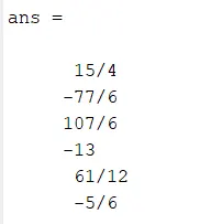
format rational was used to make sure the result is in p/q form else it may cause rounding errors later on

we get the resultant matrix which provides the solution or values of a, b, c, d, e and g

`a = 15/4`

`b=-77/6`

`c=-107/6`

`d= -13`

`e=61/12`

`g=-5/6`

Adding the 4th vertical column from Taylor's Table and we get: `f''(i)=(d^2f)/(dx^2) = (af(i) + bf(i+1) + cf(i+2)+df(i+3)+ef(i+4)+gf(i+5))/(Deltax^2)`

3. Left Skewed

To calculate number of nodes for right skewed differencing,

order of accuracy P = Number of nodes in the stencil N - order of derivative Q

we know, P = 4, Q = 2. Solving for N we get N = 6

`(d^2f)/(dx^2) = af(i) + bf(i-1) + cf(i-2)+df(i-3)+ef(i-4)+gf(i-5)`

now, a taylor's table for the same

	`f(i)`	`Deltaxf'(i)`	`Deltax^2f''(i)`	`Deltax^3f'''(i)`	`Deltax^4f''''(i)`	`Deltax^5f'''''(i)`
`af(i)`	a	0	0	0	0	0
`bf(i-1)`	b	-b	b/2	-b/6	b/24	-b/120
`cf(i-2)`	c	-2c	4c/2	-8c/6	16c/24	-32c/120
`df(i-3)`	d	-3d	9d/2	-27d/6	81d/24	-243d/120
`ef(i-4)`	e	-4e	16e/2	-64e/6	256e/24	-1024e/120
`gf(i-5)`	g	-5g	25g/2	-125g/6	625g/24	-3125g/120
	0	0	1	0	0	0

Adding the vertical columns we get,

`a+b+c+d+e+g=0`

`-b-2c-3d-4e-5g=0`

`b//2+4c//2+9d//2+16e//2+25g//2=1`

`-b//6 - 8c//6-27d//6-64e//6-125g//6=0`

`b//24-16c//24-81d/24-256e//24-625g//24=0`

`b//120-32c//120-243d//120-1024e//120-3125g//120=0`

Simplyfying some equations and arranging them into matrix form, we get

`[[1,1,1,1,1,1],[0,1,2,3,4,5],[0,1,4,9,16,25],[0,1,8,27,64,125],[0,1,16,81,256,625],[0,1,32,243,1024,3125]][[a],[b],[c],[d],[e],[g]] = [[0],[0],[2],[0],[0],[0]]`

Solving this in MATLAB using the below code,

a=[1 1 1 1 1 1;0 1 2 3 4 5;0 1 4 9 16 25; 0 1 8 27 64 125; 0 1 16 81 256 625; 0 1 32 243 1024 3125;]
b = [0 0 2 0 0 0]'
format rational
inv(a)*b

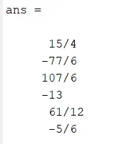
format rational was used to make sure the result is in p/q form else it may cause rounding errors later on

we get the resultant matrix which provides the solution or values of a, b, c, d, e and g

`a = 15/4`

`b=-77/6`

`c=-107/6`

`d= -13`

`e=61/12`

`g=-5/6`

Adding the 4th vertical column from Taylor's Table and we get: `f''(i)=(d^2f)/(dx^2) = (af(i) + bf(i-1) + cf(i-2)+df(i-3)+ef(i-4)+gf(i-5))/(Deltax^2)`

Calculation of Derivative

`f(x) = e^xcosx`

`f'(x) = e^x cosx - e^x sinx` - First Derivative

`f''(x) = e^x cosx - e^x sinx - e^cosx - e^x sinx`

`f''(x) = - 2 e^x sinx` Second Derivative

Code with explanation

filename: left_skew_difference.m
function error = left_skew_difference (m,analytical_second_derivative,x,dx)

% f(x)= e^x * cos(x)
% f''(x) = -2 e^x sin(x)
% left skew difference: f''(x) = a f(i) + b f(i-1) + c f(i-2)+ d f(i-3)+ e f(i-4)+ g f(i-5)
% where, a = 15/4 b=-77/6 c=-107/6 d= -13 e=61/12 g=-5/6
left_skew_derivative = (m(1)*exp(x)* cos (x) + m(2) * exp(x-dx)* cos (x-dx)+m(3)*exp(x-(2*dx))* cos (x-(2*dx))+m(4) * exp(x-(3*dx))* cos (x-(3*dx)) + m(5)* exp(x-(4*dx))* cos (x-(4*dx)) + m(6)* exp(x-(5*dx))* cos (x-(5*dx)))/(dx^2);
error = abs(left_skew_derivative-analytical_second_derivative);

end

----------
filename:right_skew_difference.m
function error = right_skew_difference (m,analytical_second_derivative,x,dx)

% f(x)= e^x * cos(x)
% f''(x) = -2 e^x sin(x)
% right skew difference f''(x) = a f(i) + b f(i+1) + c f(i+2)+ d f(i+3)+ e f(i+4)+ g f(i+5)
% where, a= 15/4, b = -77/6. c = -107/6, d=-13, e = 61/12, g = -5/6
right_skew_derivative = (m(1)*exp(x)* cos (x) + m(2) * exp(x+dx)* cos (x+dx)+m(3)*exp(x+(2*dx))* cos (x+(2*dx))+ m(4)* exp(x+(3*dx))* cos (x+(3*dx)) + m(5)* exp(x+(4*dx))* cos (x+(4*dx)) + m(6)* exp(x+(5*dx))* cos (x+(5*dx)))/(dx^2);
error = abs(right_skew_derivative-analytical_second_derivative);

end
----------
filename:central_difference.m
function error = central_difference (m,analytical_second_derivative,x,dx)

% f(x)= e^x * cos(x)
% f''(x) = -2 e^x sin(x)
% central difference f''(x) = a f(i-2) + b f(i-1) + c f(i)+ d f(i+1)+ e f(i+2)
% where, a = -1/12 b=4/3 c=-5/2 d=4/3 e=-1/12
central_derivative = (m(1)*exp(x-(2*dx))* cos (x-(2*dx)) +m(2)*exp(x-dx)*cos (x-dx) + m(3)*exp(x)* cos (x) + m(4)*exp(x+dx) * cos(x+dx) + m(5)*exp(x+(2*dx))*cos(x+(2*dx)))/(dx^2);
error = abs(central_derivative-analytical_second_derivative);

end
----------
% main program

clear all
close all
clc

format rational % to make sure rounding-off errors are minimised since we are using very small numbers

% calculating the constants for each scheme and storing in m_l,m_r and m_c
a=[1 1 1 1 1 1;0 1 2 3 4 5;0 1 4 9 16 25; 0 1 8 27 64 125; 0 1 16 81 256 625; 0 1 32 243 1024 3125;];
b = [0 0 2 0 0 0]';
m_l = inv(a)*b

a=[1 1 1 1 1 1;0 1 2 3 4 5;0 1 4 9 16 25; 0 1 8 27 64 125; 0 1 16 81 256 625; 0 1 32 243 1024 3125;];
b = [0 0 2 0 0 0]';
m_r = inv(a)*b

a=[1 1 1 1 1;-2 -1 0 1 2; 2 0.5 0 0.5 2;-4/3 -1/6 0 1/6 4/3; 2/3 1/24 0 1/24 2/3;];
b = [0 0 1 0 0]';
m_c = inv(a)*b

% function given f(x)= e^x * cos(x)
x = pi; 
dx = linspace(pi/4000,pi/3,4000); % 4000 values of dx from pi/3 to pi/4000

% analytical second derivative: f''(x) = -2 e^x sin(x)
analytical_second_derivative = -2 * exp(x) * sin(x);

% calculating left skew, right skew and central difference error for x=pi
% for each value of dx
for i = [1:length(dx)]
    
    % numerical differencing - decided to send exact derivative as a parameter so as to not calculate everytime
    
    left_skew_error (i)= left_skew_difference (m_l, analytical_second_derivative,x,dx(i));
    
    right_skew_error(i) = right_skew_difference (m_r, analytical_second_derivative,x,dx(i));
    
    central_error (i)= central_difference (m_c, analytical_second_derivative,x,dx(i));
    
end

%plotting error vs dx on a loglog plot with appropiate legends and labels
figure(1)
loglog(dx,left_skew_error,'blue')
hold on
loglog(dx,right_skew_error,'red')
hold on
loglog(dx,central_error,'black')
legend('Left Side Skewed Difference','Right Side Skewed Difference','Central Difference')
xlabel ('dx')
ylabel ('Error')

Output of Code

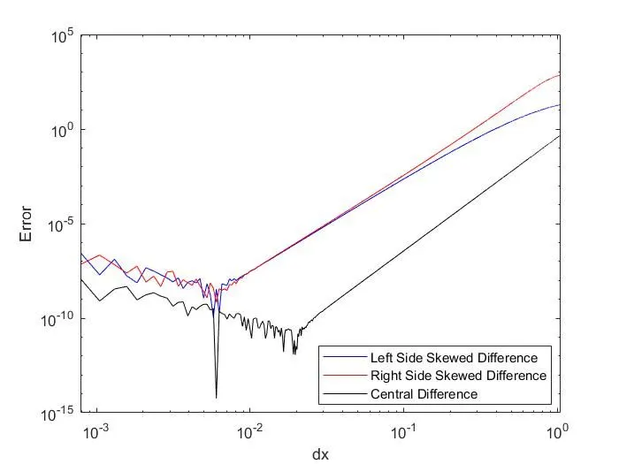
The output is a graph of the absolute errors of the 3 schemes (left, right and central) to 4000 values of dx from pi/3 to pi/4000. The graph is on a log scale for easier viewing. As expected, central difference scheme has a significantly lower error than the skewed schemes. Right and Left schemes are similar since they are almost the same for a lot of values of dx. All errors decrease with decreasing dx untill a certain point when other errors such as truncation error, roundoff errors creep in and make the solution unstable.

Q. Why a skewed scheme is useful? What can a skewed scheme do that a CD scheme cannot?

Although a central difference scheme provides lower errors for the same values of dx. Skewed schemes are useful at the boundaries of equation, which is very common in CFD (boundary conditions), a CD scheme cannot be applied at boundary conditions while a skewed scheme can be applied with relatively less error.