Simulation of a 1D Super-sonic nozzle flow simulation using Macormack Method
Simulation of a 1D Super-sonic nozzle flow simulation using Macormack Method
In this project, I will be solving a 3D nozzle flow simulation which has been converted to a 1D nozzle, disregarding any change in quantities in the y and z directions.
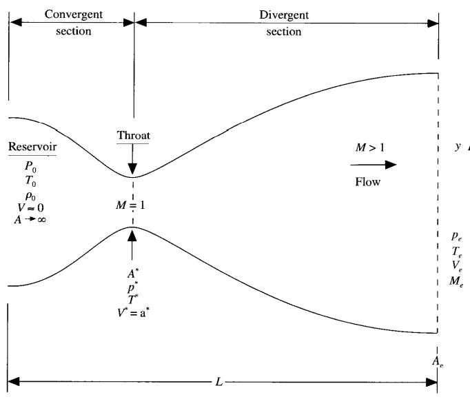
This type of flow is called quasi-one-dimensional flow.
This flow is solved using the governing equations of continuity, momentum and energy as follows:
Continuity: `underset(1)(rho)*underset(1)(V)*underset(1)(A) = underset(2)(rho)*underset(2)(V)*underset(2)(A)`
Momentum: `underset(1)(rho)*underset(1)(A) + underset(1)(rho)*underset(1)(V^2)*underset(1)(A) + int_(A1)^(A2) (p dA) = underset(2)(rho)*underset(2)(A) + underset(2)(rho)*underset(2)(V^2)*underset(2)(A) `
Energy: `underset(1)(h) + (underset(1)(V^2))/2 = underset(2)(h) + (underset(2)(V^2))/2`
These equations are solved by numerical methods in both conservative and non-conservative form.
1. Non-Conservative Form
The governing equations for the non-conservative form are as follows:
Continnuity:`(del rho')/(del t') = - rho' (del V')/(del x')- rho' V'(del ln A')/(del x')- V' (del rho')/(del x')`
Momentum: `(del V')/(del t') = - V' (del V')/(del x') - 1/gamma ((del T')/(del x')+ (T')/(rho' ) (del rho')/(del x'))`
Energy: `(del T')/(del t') = -V' (del T')/(del x') -(gamma-1)T'((del V')/(del x') +V'(del ln A')/(del x') )`
where the ' denotes that the values of all values are normalised. That is, the values are divided by a respective standard value to make the equations non-dimensionless.
where `T' = T/(underset(0)(T)), rho' = rho/(underset(0)(rho)), x' = x/L, V' = V/(underset(0)(a)), A' = A/(A^0), t' = t/(L//(underset(0)(a))`
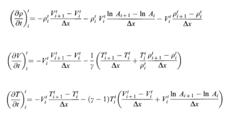
These equations are solved using the Macormack Method, which uses predictor and corrector steps to obtain a 2nd order solution.
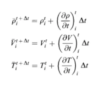
The predictor method involves solving the equations in forward differencing method, as shown below:
An intermediate solution is calculated from the predictor values
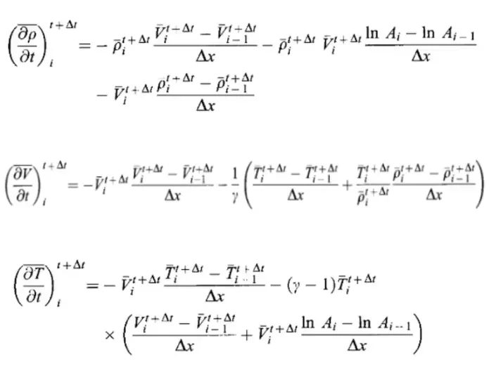
Next is the corrector step, in which the updated predicted values are backward differeced to obtain a second order solution
The corrector values and predictor values are finally averaged in this step, which gives a solution which is 2nd order accurate
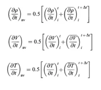
The averaged value is used to calculate final primitive values for that timestep.
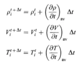
This process is repeated for all timesteps or till steady state is obtained.
Results of Non-Conversative Form
1. Steady-state distribution of primitive variables inside the nozzle
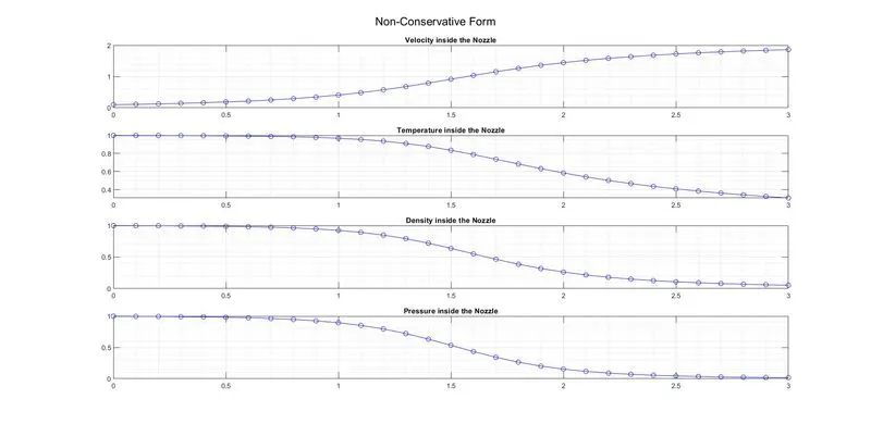
This graph shows distribution of velocity, pressure, temperature and density inside the nozzle at the final timestep (1400 in this case). We can notice that the velocity crosses 1 at x = 1.5 (throat of nozzle), the velocity transitions from subsonic to super sonic at the throat of the nozzle. The velocity gradually increases and plateau-s after a while the other values decrease gradually and plateau-s. Boundary conditions and assumptions are satisfied (velocity at inlet is 0, pressure at outlet is 0, pressure at inlet is maximum, etc.)
2. Time-wise variation of the primitive variables
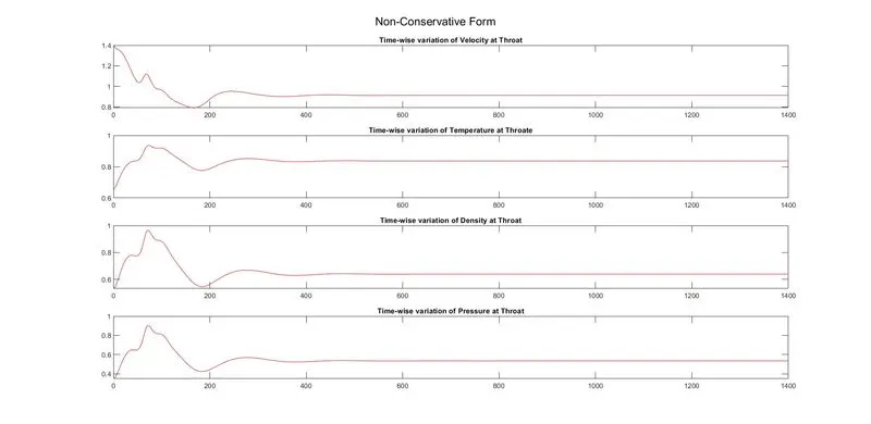
This shows the variation of velocity, temperature, density and pressure at the throat of the nozzle for all timesteps (till 1400 in this case), we can see how the solution first struggles to converge by deviating upon the true value and then finally converges at around the ~600th timestep. This devitation is expected as the nozzle requires some time to acheive steady state.
3. Variation of Mass flow rate distribution inside the nozzle at different time steps during the time-marching process
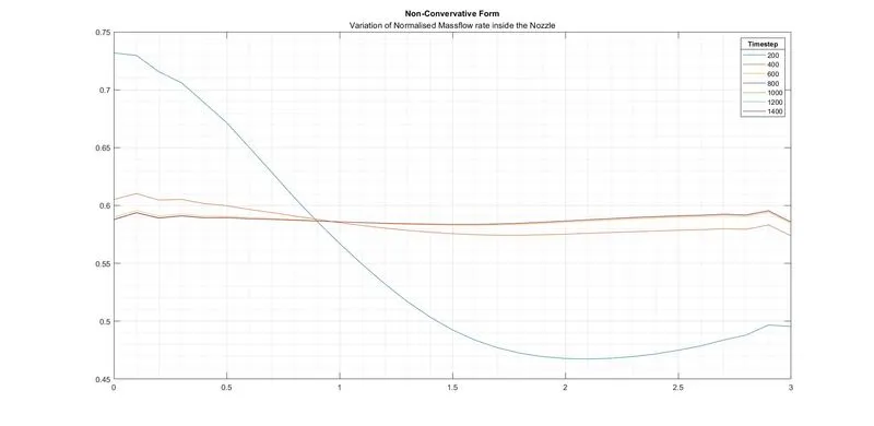
This plot shows the normalised mass flow rate across the nozzle at different timesteps, in multiples of 200. We can notice that during the earlier timesteps, the mass flow rate is quite far from the final solution, this is expected as it takes some time for steady state to occur in a system. The difference between mass flow rate at a specific timestep and final timestep decreases as the solution slowly progesses towards steady state.
Code for Non-conservative Form
% this function takes in x,n and nt as parameters and returns the mass
% profile across the nozzle during the final timestep
function [mass] = non_conservative (x,n,nt)
    dx = x(2)-x(1);

    % initial profiles for primitive variables and gamma
    rho = 1 - 0.3146*x;
    t = 1 - 0.2314*x;
    v = (0.1+1.09*x).*t.^0.5;
    gamma = 1.4;

    % calculating area
    a = 1+2.2*(x-1.5).^2;
    % finding a safe value of dt by assuming courant number as 0.5 so as to
    % have a stable solution
    dt = min(0.5*dx./(sqrt(t)+v));

    % time loop
    for k = 1:nt
        % creating copies of primitive variables
        rho_old = rho;
        v_old = v;
        t_old = t;

        % predictor loop
        for j = 2:n-1
            % instead of writing a huge expression we are splitting it
            dvdx = (v(j+1) - v(j))/dx;
            drhodx = (rho(j+1)-rho(j))/dx;
            dtdx = (t(j+1)-t(j))/dx;
            dloga_dx = (log(a(j+1)) - log(a(j)))/dx;

            % continuity equation
            drhodt_p(j) = -rho(j) * dvdx - rho(j)*v(j)*dloga_dx - v(j)*drhodx;

            % momentum equation
            dvdt_p(j) = - v(j)*dvdx - (1/gamma) * (dtdx + (t(j)*drhodx/rho(j)));

            % energy equation
            dtdt_p(j) = -v(j)*dtdx - (gamma - 1)*t(j)*(dvdx + v(j) * dloga_dx);

            % solution update
            rho(j) = rho(j) + drhodt_p(j)* dt;
            v(j) = v(j) + dvdt_p(j)* dt;
            t(j) = t(j) + dtdt_p(j)* dt;

        end

        % corrector loop
        for j = 2:n-1
            % instead of writing a huge expression we are splitting it
            dvdx = (v(j) - v(j-1))/dx;
            drhodx = (rho(j)-rho(j-1))/dx;
            dtdx = (t(j)-t(j-1))/dx;
            dloga_dx = (log(a(j)) - log(a(j-1)))/dx;

            % continuity equation
            drhodt_c(j) = -rho(j) * dvdx - rho(j)*v(j)*dloga_dx - v(j)*drhodx;

            % momentum equation
            dvdt_c(j) = - v(j)*dvdx - (1/gamma) * (dtdx + (t(j)*drhodx/rho(j)));

            % energy equation
            dtdt_c(j) = -v(j)*dtdx - (gamma - 1)*t(j)*(dvdx + v(j) * dloga_dx);
        end

        % computing the mean of predictor and corrector methods
        drhodt = 0.5 *(drhodt_p + drhodt_c);
        dvdt = 0.5 *(dvdt_p + dvdt_c);
        dtdt = 0.5 * (dtdt_p + dtdt_c);

        % final solution update
        for i = 2:n-1
            rho(i) = rho_old(i) + drhodt(i)* dt;
            v(i) = v_old(i) + dvdt(i)*dt;
            t(i) = t_old(i) + dtdt(i)*dt;
        end

        % boundary conditions
        % inlet
        v(1) = 2 * v(2) - v (3);

        % outlet
        v(n) = 2*v(n-1) - v(n-2);
        rho(n) = 2*rho(n-1) - rho(n-2);
        t(n) = 2*t(n-1) - t(n-2);

        % calculating pressure across the nozzle
        p = rho.*t;

        % calculating values for the plots at the throat
        throat = find(a==1);
        rho_throat (k) = rho(throat);
        t_throat (k) = t(throat);
        v_throat (k) = v(throat);
        p_throat (k) = p(throat);

        % calculating mass across the nozzle
        mass = rho.*a.*v;

        % plotting the mass at specific timesteps
        if rem(k,200) == 0
            figure(4)
            plot(x,mass)
            hold on
        end

    end
    % adding further details to the plot above
    figure (4)
    grid on
    grid minor
    lgd = legend('200','400','600','800','1000','1200','1400');
    title('Non-Convervative Form','Variation of Normalised Massflow rate inside the Nozzle')
    title(lgd,'Timestep')

    % plot to find time-wise variation of primitive variables at the throat
    figure (5)
    subplot (4,1,1)
    plot([1:nt],v_throat,'r')
    hold on
    title('Time-wise variation of Velocity at Throat')

    subplot (4,1,2)
    plot([1:nt],t_throat,'r')
    hold on
    title('Time-wise variation of Temperature at Throate')

    subplot (4,1,3)
    plot([1:nt],rho_throat,'r')
    hold on
    title('Time-wise variation of Density at Throat')

    subplot (4,1,4)
    plot([1:nt],p_throat,'r')
    title('Time-wise variation of Pressure at Throat')

    sgtitle('Non-Conservative Form')

    % plot to find distribution of primitive variables across the nozzle
    figure (6)
    subplot (4,1,1)
    plot(x,v,'b-o')
    grid on
    grid minor
    hold on
    title('Velocity inside the Nozzle')

    subplot (4,1,2)
    plot(x,t,'b-o')
    grid on
    grid minor
    hold on
    title('Temperature inside the Nozzle')

    subplot (4,1,3)
    plot(x,rho,'b-o')
    grid on
    grid minor
    hold on
    title('Density inside the Nozzle')

    subplot (4,1,4)
    plot(x,p,'b-o')
    grid on
    grid minor
    title('Pressure inside the Nozzle')

    sgtitle('Non-Conservative Form')

    % printing values of primitive variables at throat during the last
    % timestep for grid independence analysis
    disp('Non-Conservative Form')
    disp('Density')
    rho_throat(nt)
    disp('Temperature')
    t_throat (nt)
    disp('Pressure')
    p_throat (nt)
    disp('Velocity')
    v_throat (nt)
    disp('Mass')
    mass(throat)
    disp('Mach Number')
    v_throat (nt)/(sqrt(t_throat (nt)))
end
2. Conservative Form
The governing equations for the non-conservative form are as follows:
Continuity: `(del (rho' A'))/(del t') + (del (rho' A' V'))/(del x') = 0`
Momentum: `(del (rho' A'V'))/(del t') + (del (rho' A'V'^2 - (1//gamma)p'A'))/(del x') = 1/gamma p' (delA')/(delx')`
Energy: `(del [rho' ((e')/(gamma -1) + gamma/2 V'^2 A')]]/(del t') + (del [rho' ((e')/(gamma-1) + gamma/2 V'^2 + p'A'V')]]/(del x') = 0`
Since it is not feasible to solve such a complex solution we use subsitute some terms with solution vectors (U), flux vectors (F) and J2
where, `U1 = (rho' A'), F1 = (rho' A' V'), U2 = (rho' A' V'), F2 = (rho' A'V'^2 - (1//gamma)p'A'), J2 = 1/gamma p' (delA')/(delx'),`
`U3 = rho' ((e')/(gamma -1) + gamma/2 V'^2 A') and F3 = rho' ((e')/(gamma-1) + gamma/2 V'^2 + p'A'V')`
where the ' denotes that the values of all values are normalised. That is, the values are divided by a respective standard value to make the equations non-dimensionless.
where `T' = T/(underset(0)(T)), rho' = rho/(underset(0)(rho)), x' = x/L, V' = V/(underset(0)(a)), A' = A/(A^0), t' = t/(L//(underset(0)(a))`
This process simplyfies the conservation equations, and primitive values can be easily found
`rho' = (U1)/(A'), V' = (U2)/(U1), p'=rho'*T', T' = (gamma-1)*((U3)/(U2) - gamma/2 V'^2)`
This process provides the following equations which need to be solved now,
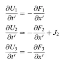
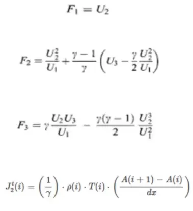
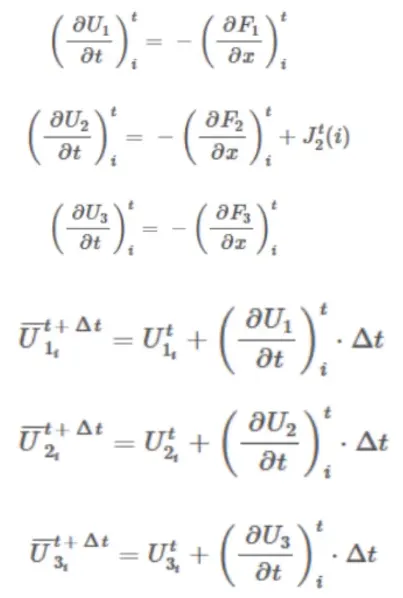
Now the predictor step values are calculated, before that the flux variables are initialised
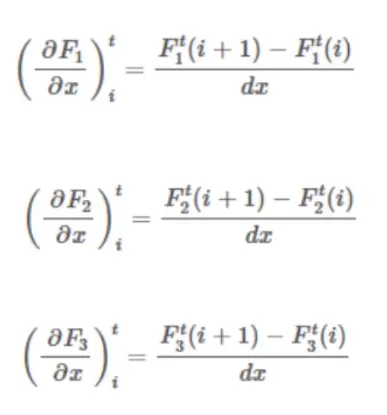
The derivative of flux values are calculated using forward differencing, as follows
The derivatives of flux values are used to find the solution vector, and predictor values of the solution are calculated
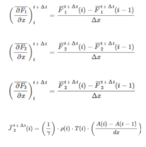
Now on to the corrector step. In this step the derivatives of the flux values are calculated using backward differencing,
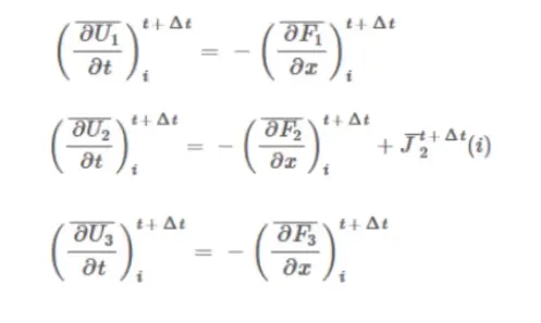
The derivatives of flux values are used to calculate the solution vectors as follows:
Then, the corrector and predictor values are averaged together to form the final 2nd order partial derivative of the solution vectors.
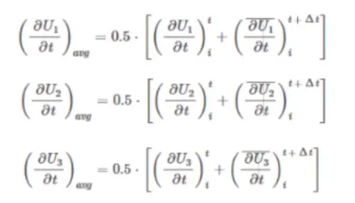
This final partial derivative is used to calculate the solution variables for that timestep.
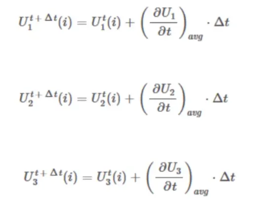
And the solution vector is reverse subsitituted, to find the values of the primitive values for that specific timestep
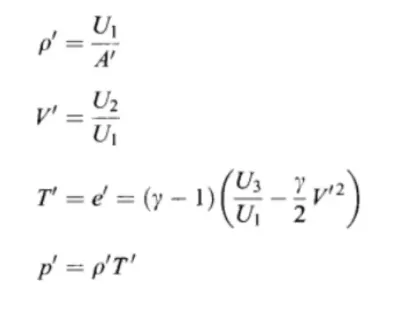
This process is repeated for all timesteps or till steady state is obtained.
Results of Conversative Form
1. Steady-state distribution of primitive variables inside the nozzle
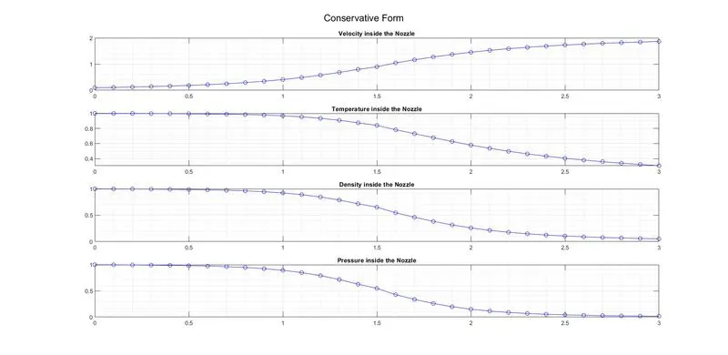
This graph shows distribution of velocity, pressure, temperature and density inside the nozzle at the final timestep (1400 in this case). We can notice that the velocity crosses 1 at x = 1.5 (throat of nozzle), the velocity transitions from subsonic to super sonic at the throat of the nozzle. The velocity gradually increases and plateau-s after a while the other values decrease gradually and plateau-s. Boundary conditions and assumptions are satisfied (velocity at inlet is 0, pressure at outlet is 0, pressure at inlet is maximum, etc.)
2. Time-wise variation of the primitive variables
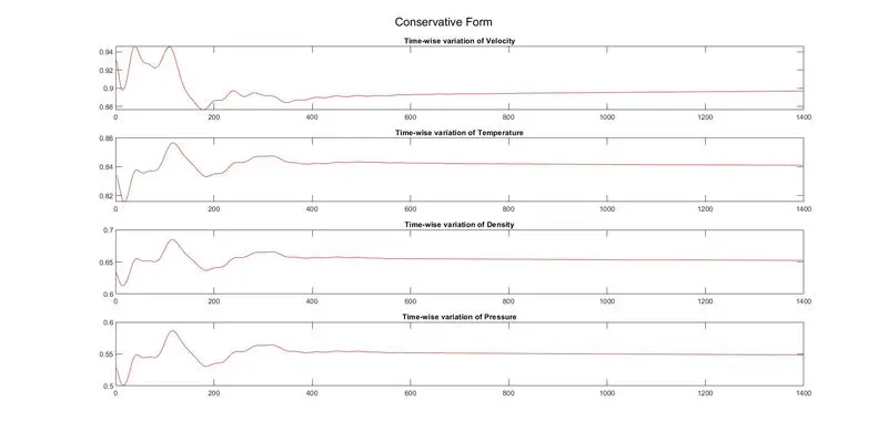
This shows the variation of velocity, temperature, density and pressure at the throat of the nozzle for all timesteps (till 1400 in this case), we can see how the solution first struggles to converge by deviating upon the true value and then finally converges at around the ~600th timestep. This devitation is expected as the nozzle requires some time to acheive steady state.
3. Variation of Mass flow rate distribution inside the nozzle at different time steps during the time-marching process
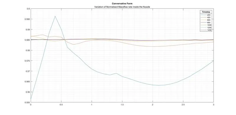
This plot shows the normalised mass flow rate across the nozzle at different timesteps, in multiples of 200. We can notice that during the earlier timesteps, the mass flow rate is quite far from the final solution, this is expected as it takes some time for steady state to occur in a system. The difference between mass flow rate at a specific timestep and final timestep decreases as the solution slowly progesses towards steady state.
Code for Conservative Form
% this function takes in x,n and nt as parameters and returns the mass
% profile across the nozzle during the final timestep
function [mass] = conservative (x,n,nt)
    dx = x(2)-x(1);

    % initial profiles for primitive variables
    % for 0 <=x <= 0.5
    rho = ones(1,n);
    t = ones(1,n);

    % for 0.5<= x <= 1.5
    for l= find(x==0.5):find(x==1.5)
        rho(l) = 1 - 0.366*(x(l)-0.5);
        t(l) = 1 - 0.167*(x(l)-0.5);
    end

    % for 1.5 <= x <= 3.5
    for l=find(x==1.5):find(x==3)
        rho(l) = 0.634 - 0.3879*(x(l)-1.5);
        t(l) = 0.833 - 0.3507*(x(l)-1.5);
    end

    % calculating area, gamma and velocity
    a = 1+2.2*(x-1.5).^2;
    v = 0.59 ./ (rho .* a);
    gamma = 1.4;

    % initialising solution variables

    u1 = rho.*a;
    u2 = rho.*a.*v;
    u3 = a.*rho.*( (t./(gamma - 1)) + (0.5 * gamma * v.^2) ) ;

    % finding a safe value of dt by assuming courant number as 0.5 so as to
    % have a stable solution
    dt = min(0.5*dx./(sqrt(t)+v));

    % time loop
    for k = 1:nt

        % intialising flux variables
        f1 = u2;
        f2 = (u2.^2./u1) + ((gamma - 1)/(gamma)) * (u3 - (0.5*gamma*u2.^2./u1));
        f3 = (gamma * u2.*u3./u1) - (0.5*gamma*(gamma-1)*u2.^3./(u1.^2));

        % creating copies of solution vectors
        u1_old = u1;
        u2_old = u2;
        u3_old = u3;

        % predictor loop
        for j = 2:n-1

            j2(j) = (1/gamma) * rho(j) * t(j) * ( (a(j+1) - a(j))/dx);
            df1dx(j) = (f1(j+1) - f1(j))/dx;
            df2dx(j) = (f2(j+1) - f2(j))/dx;
            df3dx(j) = (f3(j+1) - f3(j))/dx;

            du1dt_p(j) = -1 * df1dx(j);
            du2dt_p(j) = -1 * df2dx(j) + j2(j);
            du3dt_p(j) = -1 * df3dx(j);

            % solution vector update
            u1(j) = u1(j) + du1dt_p(j) * dt;
            u2(j) = u2(j) + du2dt_p(j) * dt;
            u3(j) = u3(j) + du3dt_p(j) * dt;
        end

        % calculating flux values for predictor updated solution vectors
        f1 = u2;
        f2 = (u2.^2./u1) + ((gamma - 1)/(gamma)) * (u3 - (0.5*gamma*u2.^2./u1));
        f3 = (gamma * u2.*u3./u1) - (0.5*gamma*(gamma-1)*u2.^3./(u1.^2));

        rho = u1./a;
        v = u2./u1;
        t = (gamma - 1)*( u3./u1 - gamma*0.5*v.^2);

        % corrector loop
        for j = 2:n-1

            j2(j) = (1/gamma) * rho(j) * t(j) * ((a(j) - a(j-1))/dx);
            df1dx(j) = (f1(j) - f1(j-1))/dx;
            df2dx(j) = (f2(j) - f2(j-1))/dx;
            df3dx(j) = (f3(j) - f3(j-1))/dx;

            du1dt_c(j) = -1 * df1dx(j);
            du2dt_c(j) = -1 * df2dx(j) + j2(j);
            du3dt_c(j) = -1 * df3dx(j);

        end

        % computing the mean of predictor and corrector methods
        du1dt= 0.5*(du1dt_p + du1dt_c);
        du2dt= 0.5*(du2dt_p + du2dt_c);
        du3dt= 0.5*(du3dt_p + du3dt_c);

        % final solution vector update
        for i = 2:n-1
            u1(i) = u1_old(i) + du1dt(i)*dt;
            u2(i) = u2_old(i) + du2dt(i)*dt;
            u3(i) = u3_old(i) + du3dt(i)*dt;
        end

        % boundary conditions
        % inlet
        u1(1) = a(1);
        u2(1) = 2*u2(2) - u2(3);
        u3(1) = u1(1).* (t(1)/(gamma-1) + 0.5*gamma*v(1)^2);

        % outlet
        u1(n) = 2*u1(n-1) - u1(n-2);
        u2(n) = 2*u2(n-1) - u2(n-2);
        u3(n) = 2*u3(n-1) - u3(n-2);

        % finding primitive values from solution vectors
        rho = u1./a;
        v = u2./u1;
        t = (gamma - 1)*( u3./u1 - gamma*0.5*v.^2);
        p = rho.*t;

        % calculating values for the plots at the throat
        throat = find(a==1);
        rho_throat (k) = rho(throat);
        t_throat (k) = t(throat);
        v_throat (k) = v(throat);
        p_throat (k) = p(throat);

        % calculating mass across the nozzle
        mass = rho.*a.*v;

        % plotting the mass at specific timesteps
        if rem(k,200) == 0
            figure(1)
            plot(x,mass)
            hold on
        end
    end
    % adding further details to the plot above
    figure (1)
    grid on
    grid minor
    lgd = legend('200','400','600','800','1000','1200','1400');
    title('Convervative Form', 'Variation of Normalised Massflow rate inside the Nozzle')
    title(lgd,'Timestep')

    % plot to find time-wise variation of primitive variables at the throat
    figure (2)
    subplot (4,1,1)
    plot([1:nt],v_throat,'r')
    hold on
    title('Time-wise variation of Velocity')

    subplot (4,1,2)
    plot([1:nt],t_throat,'r')
    hold on
    title('Time-wise variation of Temperature')

    subplot (4,1,3)
    plot([1:nt],rho_throat,'r')
    hold on
    title('Time-wise variation of Density')

    subplot (4,1,4)
    plot([1:nt],p_throat,'r')
    title('Time-wise variation of Pressure')

    sgtitle('Conservative Form')

    % plot to find distribution of primitive variables across the nozzle
    figure (3)
    subplot (4,1,1)
    plot(x,v,'b-o')
    grid on
    grid minor
    hold on
    title('Velocity inside the Nozzle')


    subplot (4,1,2)
    plot(x,t,'b-o')
    grid on
    grid minor
    hold on
    title('Temperature inside the Nozzle')

    subplot (4,1,3)
    plot(x,rho,'b-o')
    grid on
    grid minor
    hold on
    title('Density inside the Nozzle')

    subplot (4,1,4)
    plot(x,p,'b-o')
    grid on
    grid minor
    title('Pressure inside the Nozzle')

    sgtitle('Conservative Form')

    % printing values of primitive variables at throat during the last
    % timestep for grid independence analysis
    disp('Conservative Form')
    disp('Density')
    rho_throat(nt)
    disp('Temperature')
    t_throat (nt)
    disp('Pressure')
    p_throat (nt)
    disp('Velocity')
    v_throat (nt)
    disp('Mass')
    mass(throat)
    disp('Mach Number')
    v_throat (nt)/(sqrt(t_throat (nt)))

end
Comparison of Normalized mass flow rate distributions of both forms
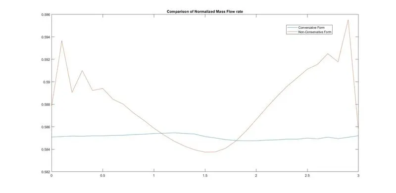
This plot shows the normalised mass flow rate across the nozzle at the final timestep (1400 in this case) when the solution has attained steady state for both Conservative and Non-Conservative forms. We can notice that the conservative form is more smooth, while the non-conservative form seems jagged. Keep in mind, that the y-axis scale is very small, so small differences in mass flow rate appear more magnified in this case. The jagged-ness could be explained by assuming the solution is about to become unstable for the non-conservative form.
Main Program Code
clear all
close all
clc

% inputs
n = 31;
x = linspace(0,3,n);
nt = 1400;

% these functions takes in x,n and nt as parameters and returns the mass
% profile across the nozzle during the final timestep

mass_c = conservative (x,n,nt);

mass_nc = non_conservative (x,n,nt);

% to plot variation of mass across nozzle for both forms
figure(7)
plot(x,mass_c)
hold on
plot(x,mass_nc)
legend('Conversative Form','Non-Conservative Form')
title ('Comparison of Normalized Mass Flow rate')
Grid Independence Test
In order to check if the solution is independent of the number of grid points used, a grid independence test was performed to ensure the solution's tenability. The number of grid divisions were increased to 60 (increasing grid points to 61) and the result are below:
| Number of Gridpoints | `rho'` | `T'` | `p'` | `V'` | `m'` | `M` |
| Case 1: 31 points | 0.6387 | 0.8365 | 0.5342 | 0.9140 | 0.5838 | 0.9994 |
| Case 2: 61 points | 0.6377 | 0.8354 | 0.5327 | 0.9138 | 0.5827 | 0.9998 |
| Analytical Solution* | 0.634 | 0.833 | 0.528 | 0.914 | 0.579 | 1.000 |
The values listed above are at the throat of the nozzle at the final timestep for non-conservative form (1400 in this case)
* - The analytical solution was taken from Computational Fluid Dynamics: The Basics with Applications, John David Anderson, Table 7.5 - Page 323
We can notice that the solution does not gain any significant improvement in precision when the number of gridpoints is increased. We can conlcude from this that the solution is independent of the number of grid points used. If further precision is required for complex applications, the grid size can be increase appropriately. Do note this increase will definitely cause an increase in simulation time for more complex simulations.