Week 5.1 - Mid term project - Solving the steady and unsteady 2D heat conduction problem
Steady state is referred to when the temperature with respect to time does not change.
Unsteady/Transient State is shen the temperature with respect to time does change.
The 2nd order partial diffential equation for Unsteady State is:
`(delta T)/(delta t) - alpha *((delta^2T)/(delta x^2) + (delta^2T)/(delta y^2)) = 0`
During steady state, `(delta T)/(delta t) = 0`
hence the equation becomes,
`(delta^2T)/(delta x^2) + (delta^2T)/(delta y^2) = 0`
We solve the equations in a total of 7 ways:
1. Steady State - Jacobi Method
this is the PDE to be solved.
`(delta^2T)/(delta x^2) + (delta^2T)/(delta y^2) = 0`
discretising this and rearranging the terms, we get:
`underset (P)(T) = 1/k ((underset(L)(T)+underset(R)(T))/(Delta x^2)) + 1/k ((underset(T)(T)+underset(B)(T))/(Delta y^2))`
where `k = 2((Delta x^2+Delta y^2)/(Delta x^2* Delta y^2))`
here, the values of T on the right hand side are the values of the previous iteration and not the current iteration
Function code which takes dx, dy, nx, ny, T, error and tolerance as arguments
filename: steady_jacobi_solver.m
function [T,jacobi_iterations] = steady_jacobi_solver (dx, dy,nx,ny,T,error,tol)
    % creating copy of solution array
    Told = T;
    k = 2 * ( (dx^2 + dx^2)/(dx*dy)^2);
    jacobi_iterations = 1;
    % convergence loop
    while(error>tol)
            for i = 2:nx-1
                for j = 2:ny-1
                    T(i,j)=((Told(i-1,j) + Told(i+1,j))/(k*dx^2)) + ((Told(i,j-1) + Told(i,j+1))/(k*dy^2));
                end
            end
        % calculating error and updating Told
        error = max(max(abs(Told- T)));
        Told = T;
        jacobi_iterations = jacobi_iterations + 1;
    end
end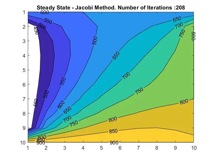
Figure shows a filled contour plot of the temperature distribution in the domain calculated by a Jacobi solver for steady state. As expected, the boundary conditions (bottom: 900K, left: 400K, right: 800K and top: 600K) are satisfied
2. Steady State - Gauss Seidel Method
this is the PDE to be solved.
`(delta^2T)/(delta x^2) + (delta^2T)/(delta y^2) = 0`
discretising this and rearranging the terms, we get:
`underset (P)(T) = 1/k ((underset(L)(T)+underset(R)(T))/(Delta x^2)) + 1/k ((underset(T)(T)+underset(B)(T))/(Delta y^2))`
where `k = 2((Delta x^2+Delta y^2)/(Delta x^2* Delta y^2))`
here, the values of T on the right hand side are the values of the current iteration and not the previous iteration
Function code which takes dx, dy, nx, ny, T, error and tolerance as arguments
filename:steady_gauss_seidel_solver.m
function [T,gs_iterations] = steady_gauss_seidel_solver (dx, dy,nx,ny,T,error,tol)
    % creating copy of solution array
    Told = T;
    k = 2 * ( (dx^2 + dx^2)/(dx*dy)^2);
    gs_iterations = 1;
    % convergence loop
    while(error>tol)
            for i = 2:nx-1
                for j = 2:ny-1
                    T(i,j)=((T(i-1,j) + T(i+1,j))/(k*dx^2)) + ((T(i,j-1) + T(i,j+1))/(k*dy^2));
                end
            end
        % calculating error and updating Told
        error = max(max(abs(Told- T)));
        Told = T;
        gs_iterations = gs_iterations + 1;
     end
end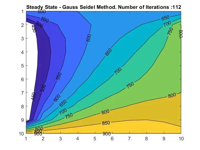
Figure shows a filled contour plot of the temperature distribution in the domain calculated by a Gauss Seidel solver for steady state. As expected, the boundary conditions (bottom: 900K, left: 400K, right: 800K and top: 600K) are satisfied
3. Steady State - Succesive over relaxation Method
this is the PDE to be solved.
`(delta^2T)/(delta x^2) + (delta^2T)/(delta y^2) = 0`
discretising this, rearranging the terms and applying succiesive over relaxation for gauss seidel, we get:
`underset(P)(T^(n+1)) = (1-omega) overset(n)(T) + omega * ( 1/k ((underset(L)(T)+underset(R)(T))/(Delta x^2)) + 1/k ((underset(T)(T)+underset(B)(T))/(Delta y^2)))`
where `omega` is the relaxation factor
w > 1 overrelaxed
w < 1 underrelaxed
and `k = 2((Delta x^2+Delta y^2)/(Delta x^2* Delta y^2))`
here, the values of T on the right hand side are the values of the current iteration and not the previous iteration
Function code which takes dx, dy, nx, ny, T, error and tolerance as arguments
filename:steady_sor_solver.m
function [T,sor_iterations] = steady_sor_solver (dx, dy,nx,ny,T,error,tol)
    % creating copy of solution array
    Told = T;
    k = 2 * ( (dx^2 + dx^2)/(dx*dy)^2);
    w = 1.2; % relaxation factor or 1.2
    sor_iterations = 1;
    % convergence loop
    while(error>tol)
            for i = 2:nx-1
                for j = 2:ny-1
                    T(i,j)=(1-w)*(Told(i,j))+w*(((T(i-1,j) + T(i+1,j))/(k*dx^2)) + ((T(i,j-1) + T(i,j+1))/(k*dy^2)));
                end
            end
        % calculating error and updating Told
        error = max(max(abs(Told- T)));
        Told = T;
        sor_iterations = sor_iterations + 1;
    end
end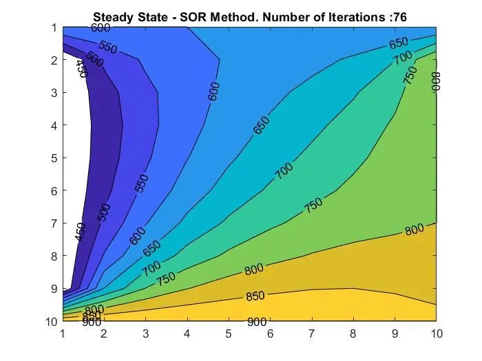
Figure shows a filled contour plot of the temperature distribution in the domain calculated by a succesive relaxation solver for gauss seidel steady state. As expected, the boundary conditions (bottom: 900K, left: 400K, right: 800K and top: 600K) are satisfied
4. Unsteady State - Explicit
this is the PDE to be solved.
`(delta T)/(delta t) - alpha *((delta^2T)/(delta x^2) + (delta^2T)/(delta y^2)) = 0`
discretising this and rearranging the terms, we get:
`underset (P)(T^(n+1)) = underset(P)(T^n)+ underset (1)(k) * (underset(L)(T) - 2* underset(P)(T) +underset(R)(T)) ^n + underset(2)(k)*(underset(T)(T) - 2* underset(P)(T) +underset(B)(T)) ^n`
where `alpha` is the heat transfer coefficient, `underset(1)(k) = (alpha Delta t )/ (Delta x^2)` and `underset(2)(k) = (alpha Delta t )/ (Delta y^2)`
Note: the exponent `n` denotes that this takes place in the n th timestep
here, the values of T on the right hand side are the values of the previous timestep and not the current timestep
Function code which takes dx, dy, nx, ny and T as arguments
filename: unsteady_explicit_solver.m
function [T,explicit_iterations] = unsteady_explicit_solver (dx, dy,nx,ny,T)
    % initial conditions
    dt = 1e-3;
    alpha = 1.4;
    k1 = alpha * dt / dx^2;
    k2 = alpha * dt / dy^2;

    explicit_iterations = 1;
    nt = 1400;
    % time loop
    for k = 1:nt
        % convergence loop
        for i = 2:nx-1
            for j = 2:ny-1
                T(i,j)= T(i,j) + k1 *(T(i-1,j) - 2*T(i,j) + T(i+1,j)) + k2 * (T(i,j-1) - 2*T(i,j) + T(i,j+1));
            end
        end
        explicit_iterations = explicit_iterations + 1;
    end
end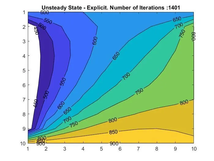
Figure shows a filled contour plot of the temperature distribution in the domain calculated by an explicit solver for unsteady state. As expected, the boundary conditions (bottom: 900K, left: 400K, right: 800K and top: 600K) are satisfied
5. Unsteady State - Implicit - Jacobi Solver
this is the PDE to be solved.
`(delta T)/(delta t) - alpha *((delta^2T)/(delta x^2) + (delta^2T)/(delta y^2)) = 0`
discretising this and rearranging the terms, we get:
`underset(P)(T^(n+1)) = (1/(1+2*k1 + 2*k2)) * ( underset(P)(T^(n)) + k1 *(underset(L)(T) + underset(R)(T))^(n+1) + k2* (underset(T)(T) + underset(B)(T))^(n+1))`
where `alpha` is the heat transfer coefficient, `underset(1)(k) = (alpha Delta t )/ (Delta x^2)` and `underset(2)(k) = (alpha Delta t )/ (Delta y^2)`
Note: the exponent `n+1` denotes that this takes place in the n+1 th timestep
here, the values of T on the right hand side are the values of the previous iteration and not the current iteration
Function code which takes dx, dy, nx, ny, T, error and tolerance as arguments
filename: unsteady_jacobi_solver.m
function [T,unsteady_jacobi_iterations] = unsteady_jacobi_solver (dx, dy,nx,ny,T,error,tol)
    % creating copies of solution array
    T_prev_dt = T;
    Told = T;

    % initial conditions
    dt = 1e-3;
    alpha = 1.4;

    k1 = alpha * dt / dx^2;
    k2 = alpha * dt / dy^2;
    unsteady_jacobi_iterations = 1;
    nt = 1400;
    % Time loop
    for k = 1:nt
        % convergence loop
        while(error>tol)
            for i = 2:nx-1
                for j = 2:ny-1
                    T(i,j)= (1/(1+2*k1+2*k2)) * ( T_prev_dt(i,j) +( k1 * (Told(i-1,j) + Told (i+1,j))) +( k2 * (Told (i,j-1) + Told (i,j+1))));
                end
            end
            % calculating error and updating Told
            error = max(max(abs(Told- T)));
            Told = T;
            unsteady_jacobi_iterations = unsteady_jacobi_iterations + 1;
        end
        % resetting error and updating T of previous time step
        T_prev_dt = T;
        error = 1;
    end
end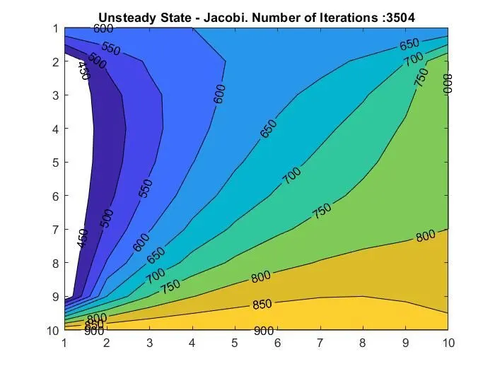
Figure shows a filled contour plot of the temperature distribution in the domain calculated by a jacobi solver for unsteady state. As expected, the boundary conditions (bottom: 900K, left: 400K, right: 800K and top: 600K) are satisfied
6. Unsteady State - Implicit - Gauss Seidel Solver
this is the PDE to be solved.
`(delta T)/(delta t) - alpha *((delta^2T)/(delta x^2) + (delta^2T)/(delta y^2)) = 0`
discretising this and rearranging the terms, we get:
`underset(P)(T^(n+1)) = (1/(1+2*k1 + 2*k2)) * ( underset(P)(T^(n)) + k1 *(underset(L)(T) + underset(R)(T))^(n+1) + k2* (underset(T)(T) + underset(B)(T))^(n+1))`
where `alpha` is the heat transfer coefficient, `underset(1)(k) = (alpha Delta t )/ (Delta x^2)` and `underset(2)(k) = (alpha Delta t )/ (Delta y^2)`
Note: the exponent `n+1` denotes that this takes place in the n+1 th timestep
here, the values of T on the right hand side are the values of the current iteration and not the previous iteration
Function code which takes dx, dy, nx, ny, T, error and tolerance as argument
filename: unsteady_sor_solver.m
function [T,unsteady_sor_iterations] = unsteady_sor_solver (dx, dy,nx,ny,T,error,tol)
    % creating copies of solution array
    T_prev_dt = T;
    Told = T;

    % initial conditions
    dt = 1e-3;
    alpha = 1.4;
    w = 1.1; % relaxation factor or 1.2
    k1 = alpha * dt / dx^2;
    k2 = alpha * dt / dy^2;
    unsteady_sor_iterations = 1;
    nt = 1400;
    % time loop
    for k = 1:nt
        % convergence loop
        while(error>tol)
            for i = 2:nx-1
                for j = 2:ny-1
                    T(i,j)= (1-w)*(Told(i,j))+w*((1/(1+2*k1+2*k2)) * ( T_prev_dt(i,j) +( k1 * (T(i-1,j) + T (i+1,j))) +( k2 * (T (i,j-1) + T (i,j+1)))));
                end
            end
            % calculating error and updating Told
            error = max(max(abs(Told- T)));
            Told = T;
            unsteady_sor_iterations = unsteady_sor_iterations + 1;
        end
        % resetting error and updating T of previous time step
        T_prev_dt = T;
        error = 1;
    end
end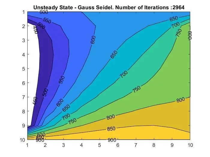
Figure shows a filled contour plot of the temperature distribution in the domain calculated by a gauss seidel solver for unsteady state. As expected, the boundary conditions (bottom: 900K, left: 400K, right: 800K and top: 600K) are satisfied
7. Unsteady State - Implicit - Succesive over relaxation solver
this is the PDE to be solved.
`(delta T)/(delta t) - alpha *((delta^2T)/(delta x^2) + (delta^2T)/(delta y^2)) = 0`
discretising this, rearranging the terms and applying succiesive over relaxation for gauss seidel, we get:
`underset(P)(T^(n+1)) = (1-omega) overset(n)(T) + omega * ((1/(1+2*k1 + 2*k2)) * ( underset(P)(T^(n)) + k1 *(underset(L)(T) + underset(R)(T))^(n+1) + k2* (underset(T)(T) + underset(B)(T))^(n+1)))`
where `alpha` is the heat transfer coefficient, `omega` is the relaxation factor`underset(1)(k) = (alpha Delta t )/ (Delta x^2)` and `underset(2)(k) = (alpha Delta t )/ (Delta y^2)`
w > 1 overrelaxed
w < 1 underrelaxed
Note: the exponent `n+1` denotes that this takes place in the n+1 th timestep
here, the values of T on the right hand side are the values of the current iteration and not the previous iteration
Function code which takes dx, dy, nx, ny, T, error and tolerance as argument
filename: unsteady_sor_solver.m
function [T,unsteady_sor_iterations] = unsteady_sor_solver (dx, dy,nx,ny,T,error,tol)
    % creating copies of solution array
    T_prev_dt = T;
    Told = T;

    % initial conditions
    dt = 1e-3;
    alpha = 1.4;
    w = 1.1; % relaxation factor or 1.2
    k1 = alpha * dt / dx^2;
    k2 = alpha * dt / dy^2;
    unsteady_sor_iterations = 1;
    nt = 1400;
    % time loop
    for k = 1:nt
        % convergence loop
        while(error>tol)
            for i = 2:nx-1
                for j = 2:ny-1
                    T(i,j)= (1-w)*(Told(i,j))+w*((1/(1+2*k1+2*k2)) * ( T_prev_dt(i,j) +( k1 * (T(i-1,j) + T (i+1,j))) +( k2 * (T (i,j-1) + T (i,j+1)))));
                end
            end
            % calculating error and updating Told
            error = max(max(abs(Told- T)));
            Told = T;
            unsteady_sor_iterations = unsteady_sor_iterations + 1;
        end
        % resetting error and updating T of previous time step
        T_prev_dt = T;
        error = 1;
    end
end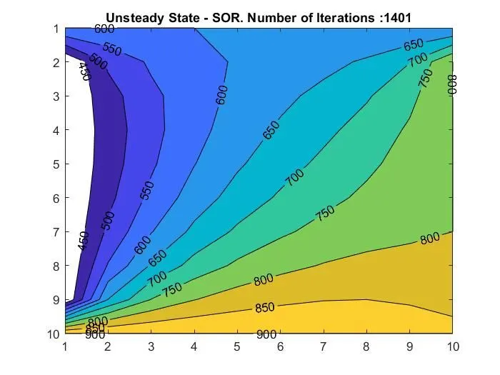
Figure shows a filled contour plot of the temperature distribution in the domain calculated by succesive overrelaxation for gauss seidel for unsteady state. As expected, the boundary conditions (bottom: 900K, left: 400K, right: 800K and top: 600K) are satisfied.
Conclusions and Observations
| State of Domain | Method Used | Number of Iterations |
| Steady State | Jacobi | 208 |
| Steady State | Gauss Seidel | 112 |
| Steady State | Succesive Overrelaxation | 76 |
| Unsteady State | Explicit | 1401 |
| Unsteady State | Jacobi | 3504 |
| Unsteady State | Gauss Seidel | 2964 |
| Unsteady State | Succesive Overrelaxation | 1401 |
We can notice that steady state solutions convergence significantly faster than unsteady state equations, this is because steady state equations are more simple than unsteady equations.
We can also notice a pattern between the 3 solvers, both in steady and unsteady states. Jacobi solvers take the most number of iterations, followed by gauss seidel and then succesive overrelaxation.
The decrease in iterations is also not linear, it seems to follow an exponential decrease
Main Function
clear all
close all
clc

nx = 10; % gridpoints alon x more gridpoints makes more iterations
ny = nx;
L = 1;

% initial conditions top = 600K bottom = 900K left = 400K right = 800K

T = 300*ones(nx);
T(:,1) = 400;
T(:,nx) = 800;
T(1,:) = 600;
T(nx,:) = 900;

% generating nodes and grid spacing
x = linspace (0,1,nx+1);
y = linspace(0,1,ny+1);
dx = L/(nx);
dy = L/(ny);

% predetermined error and tolerance
error = 1;
tol = 1e-4;

% these functions calculate the solution array and number of iterations
% used. they take dx, dy, nx, ny, T, error and tolerance as arguments
[T_solution,i] = steady_jacobi_solver (dx, dy,nx,ny,T,error,tol);
figure(1)
contourf(T_solution,[450:50:900],'ShowText','on')
title(['Steady State - Jacobi Method. Number of Iterations :',num2str(i)])
set(gca,'YDIR','reverse')

[T_solution,i] = steady_gauss_seidel_solver (dx, dy,nx,ny,T,error,tol);
figure(2)
contourf(T_solution,[450:50:900],'ShowText','on')
title(['Steady State - Gauss Seidel Method. Number of Iterations :',num2str(i)])
set(gca,'YDIR','reverse')

[T_solution,i] = steady_sor_solver (dx, dy,nx,ny,T,error,tol);
figure(3)
contourf(T_solution,[450:50:900],'ShowText','on')
title(['Steady State - SOR Method. Number of Iterations :',num2str(i)])
set(gca,'YDIR','reverse')

[T_solution,i] = unsteady_explicit_solver (dx, dy,nx,ny,T);
figure(4)
contourf(T_solution,[450:50:900],'ShowText','on')
title(['Unsteady State - Explicit. Number of Iterations :',num2str(i)])
set(gca,'YDIR','reverse')

[T_solution,i] = unsteady_jacobi_solver (dx, dy,nx,ny,T,error,tol);
figure(5)
contourf(T_solution,[450:50:900],'ShowText','on')
title(['Unsteady State - Jacobi. Number of Iterations :',num2str(i)])
set(gca,'YDIR','reverse')

[T,i] = unsteady_gauss_seidel_solver (dx, dy,nx,ny,T,error,tol);
figure(6)
contourf(T_solution,[450:50:900],'ShowText','on')
title(['Unsteady State - Gauss Seidel. Number of Iterations :',num2str(i)])
set(gca,'YDIR','reverse')

[T,i] = unsteady_sor_solver (dx, dy,nx,ny,T,error,tol);
figure(7)
contourf(T_solution,[450:50:900],'ShowText','on')
title(['Unsteady State - SOR. Number of Iterations :',num2str(i)])
set(gca,'YDIR','reverse')