Week 8 - Simulating Cyclone separator with Discrete Phase Modelling

Aim:-

To perform analysis on cyclone separator and calculate the separation efficiency and pressure drop.

Objective:-

1. To write a few words about any four empirical models used to calculate the cyclone separator efficiency.
2. To perform an analysis on a given cyclone separator model by varying the particle diameter from 1 μm to 5 μm and calculate the separation efficiency in each case. Discuss the results. [Use both the velocity's as 3m/sec.]
3. To perform an analysis on a given cyclone separator model by varying the particle velocity from 1 m/sec to 5 m/sec and calculate the separation efficiency and pressure drop in each case. Discuss the results. [Use particle diameter size as 5 μm for all cases & keep flow velocity same as particle velocity]

Introduction:

cyclone separation is a method of removing the particulates from an air, gas or liquid stream without using filters through vortex separation. when removing particulate matter from the liquid stream, use hydro cyclone. while for the gas stream, use a gas cyclone.

rotational effect and gravity effect are used to separate the mixture of solid and fluid.

A high speed rotating airflow is established within a cylindrical or conical container called a cyclone. air flows in a helical pattern, beginning from the top (wider end) of the cyclone and ending from the bottom (narrow end). the larger(denser) particles have too much inertia to follow the tight curve of the stream and thus strike the outside wall and then fall to the bottom of the cyclone where they can be removed.

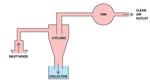
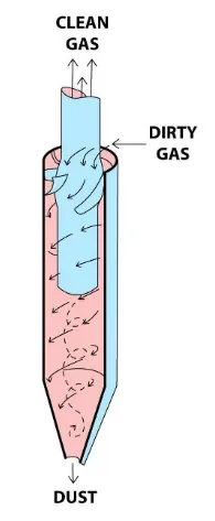
Figure: Typical gas cyclone installation Figure: Reverse flow cyclone separator

Cyclone Theory:

As the cyclone is essentially a two-phase particle-fluid system, fluid mechanics and particle transport equations are used to describe the behaviour of cyclones. the air in the cyclone enters tangentially with a velocity `V_i`. Assuming that particles are spherical in shape, a simple analysis to calculate the critical separation particles size can be established.

Let, r=rotational radius of the cyclone from the central axis. particle is subjected to three forces: Drag force (`F_d`), Bouncy force (`F_b`) and centrifugal force (`F_c`).

Fluid velocity= tengential velocity component +radially outward velocity component

`V_i=V_t+V_r`

Drag force`(F_d)`:

Stokes law: drag force exerted on a spherical object with very small Reynolds numbers in a viscous fluid.

`F_d=6pimur_p V_r`

Centrifugal force `(F_c)`:

`F_c=mromega^2`

`F_c=mV_t^2/r`

`F_c=rho_p 4/3pir_p^3 V_t^2/r`

Buoyant force (`F_b`):

the buoyant force acts in a radially inward direction which is opposite to drag force which means centripetal force.

`F_b=-rho_f 4/3pir_p^3V_t^2/r`

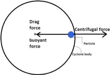
Figure: forces on partical in cyclone

Newton second law of motion: To determine the ouward radial motion of each partical.

Net Force, F=ma

`F_d+F_b+F_c=m(dV_r)/(dt)`

To simplyfy the analysis, we consider that the partical has reached its terminal velocity, i.e. its acceleration is zero

`F_d+F_b+F_c=0`

`6pimur_p V_r-rho_f 4/3pir_p^3V_t^2/r+rho_p 4/3pir_p^3 V_t^2/r=0`

`V_r=2/9 r_p^2/muV_t^2/r(rho_p-rho_f)`

Separation efficiency:

it is also known as the recovery rate or capture rate. it is the measurement of a cyclone's ability to separate the particles from the flowing gas stream.

`eta_(seperation)=` No. of Particles tracked/ No. of Particles traped

Cut point:

it is the point at which particles are removed from the gas stream at 50% efficiency.

Pressure drop:

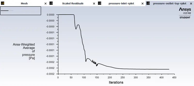
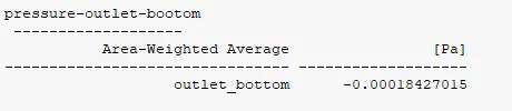
Pressure drop = pressure at inlet-pressure at outlet top

Factors affecting efficiency:

1. Particle Density: Dense particulates such as ferrous oxides can be separated with a 99% or greater efficiency, irrespective of particle size. When the particle density decreases, the efficiency decreases.

1. Particle size: Larger particles can be more easily separated than smaller particles. Particles smaller than five microns are difficult to separate without using very small separators. Particles exceeding 200 microns can often be separated using other means such as gravity-settling chambers. A reduction in particle size will give a corresponding reduction in inefficiency.

Discrete phase:

There are two approaches to the numerical calculation of multiphase flows.

1. First approach: Euler-Lagrange approach
2. Second approach: Euler-Euler approach

1. Euler-Lagrange approach:

The Lagrangian discrete phase model in ANSYS FLUENT follows the Euler-Lagrange approach. The fluid phase is treated as a continuum by solving Navier-stokes equations. while the dispersed phase is solved by tracking a large number of particles, bubbles or droplets through a calculated flow field. The dispersed phase can exchange mass, momentum and energy with the fluid phase.

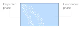
The fundamental assumption in this is that the dispersed second phase occupies a low volume fraction. the particle or droplet trajectories are computed individually at specified intervals during the fluid phase calculation. this makes the model appropriate for modelling spray dryers (produce dry powder from liquid), coal and liquid fuel combustion. but inappropriate for modelling of a liquid-liquid mixture, fluidised bed and any application where the volume fraction of the second phase can not be neglected.

Cyclone efficiency Empirical model:

models to predict the behaviour of cyclones are usually empirical. it remains largely a process of trial and error since empirical models are applicable to the only specific geometry of cyclones. four different cyclone efficiency empirical models are:

1. Iozia and Leith
2. Li and Wang
3. Koch and Licht
4. Lapple

Iozia and Leith model:

`eta=1/(1+(d_(pc)/d_(p_i))^beta`

where,

`d_(pc)`=cut particle diameter collected with 50 % efficiency (m)

`d_(p_i)`= particle diameter in size range i (m)

`beta`= slop parameter (it is a expression derived from statistical analysis of experimental data)

Li and Wang model:

• Assumptions:

1. The radial particle velocity and the radial concentration profile are not constant for uncollected particles within the cyclone.
2. The tangential velocity is related to the radius of the cyclone by uRn = constant.

Koch and Licht model:

• Assumptions:

1. The tangential velocity of a particle is equal to the tangential velocity of the gas flow, i.e. there is no slip in the tangential direction between the particle and the gas
2. The tangential velocity is related to the radius of the cyclone by uRn = constant.

Lapple model:

• Assumptions:

1. Lapple assumed that a particle entering the cyclone is evenly distributed across the inlet opening
2. The particle that travels from the inlet half-width to the wall in the cyclone is collected with 50% efficiency.

Simulation steps:

1. Geometry

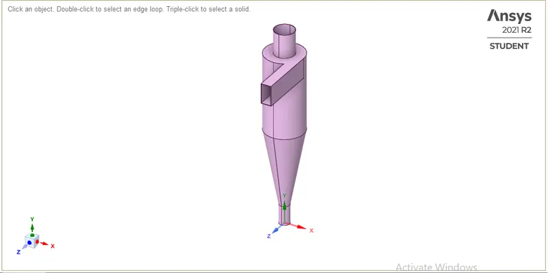
Figure: Imported geometry in SpaceClaim

Now we extract fluid volume. so to extract fluid volume, will follow the following steps

1. Prepare

2. Volume Extract

3. Select Edges

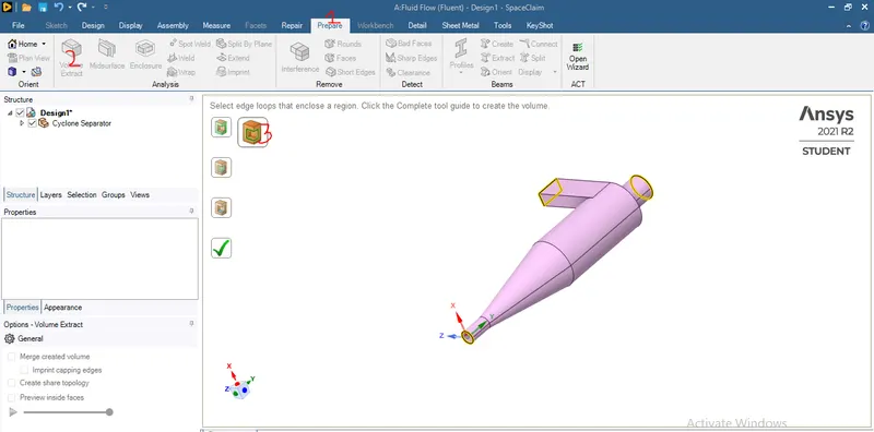
Figure: Selected edges to create fluid volume

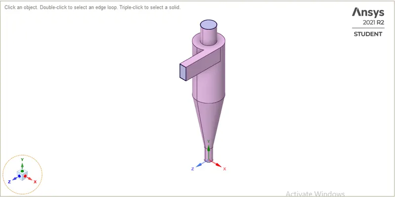
Figure: Created Fluid Volume

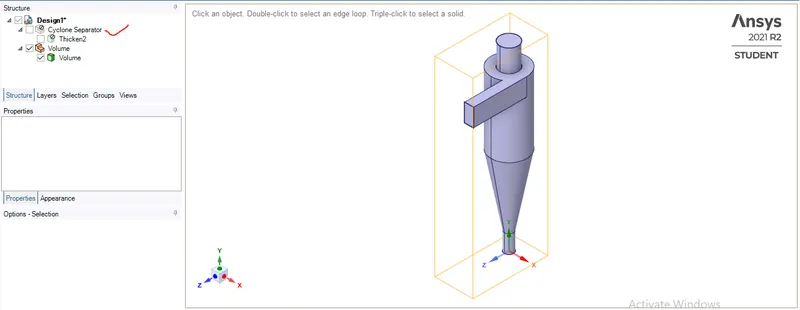
Figure: Suppressed cyclone separator geometry

Step 2. Mesh:

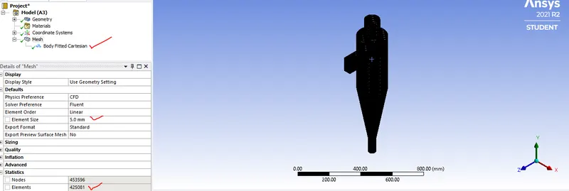
Figure: refined mesh

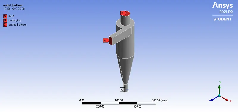
Figure: Named Selection

Step 3: Setup

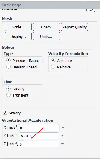
Figure: gravitational force is acting in a negative Y direction.

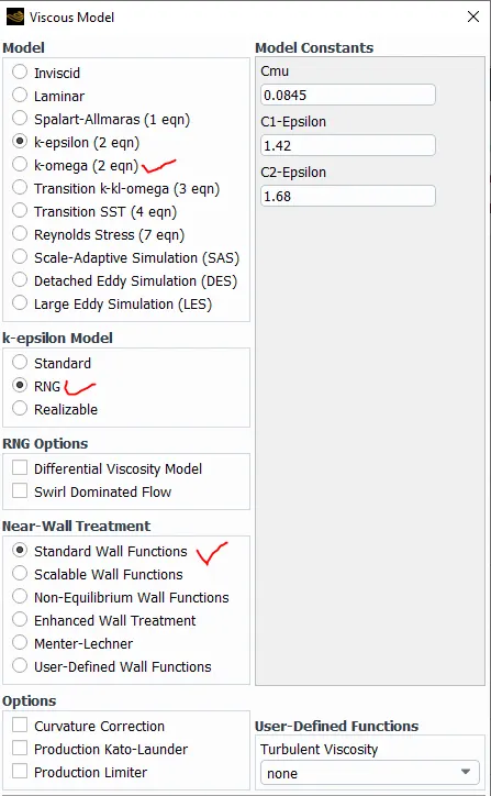
Figure: Model selection

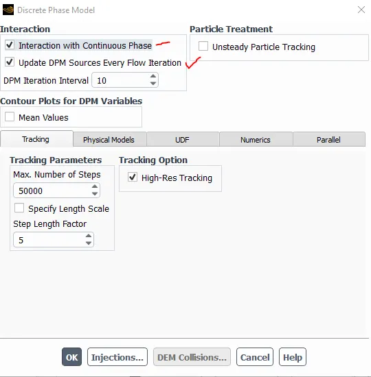
Figure: Discrete phase model

Objective 2(a) : Diameter=1 micrometer, velocity=3m/s

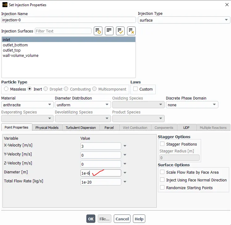
Figure: Injection properties

Discrete phase boundary condition Type:

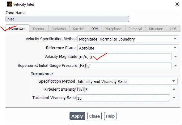
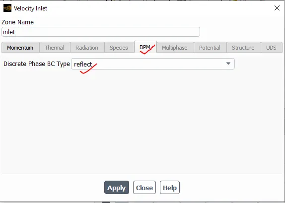
Figure: Inlet boundary condition

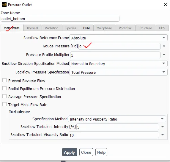
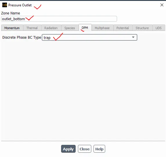
Figure: Outlet_bottom boundary condition

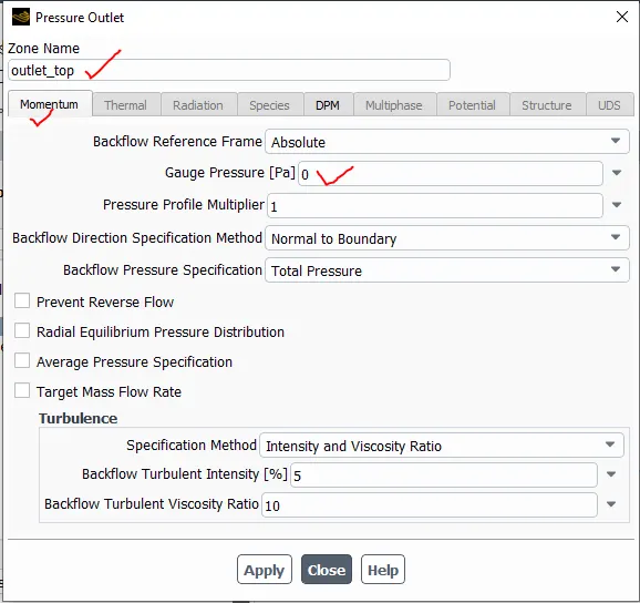
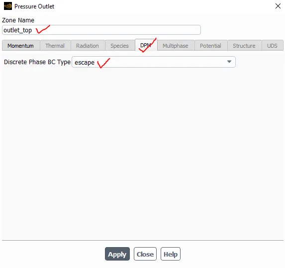
Figure: Outlet_top boundary condition

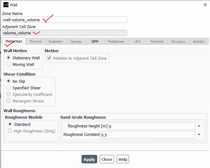
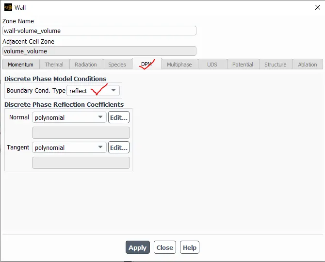
Figure: Wall-volume_volume boundary condition

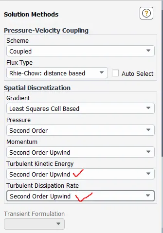
Figure: Solution method

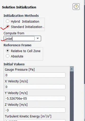
Figure: Solution initialization

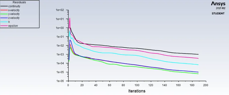
Figure: Residual plot

Figure: Convergence

`eta=235/378=0.62=62%`

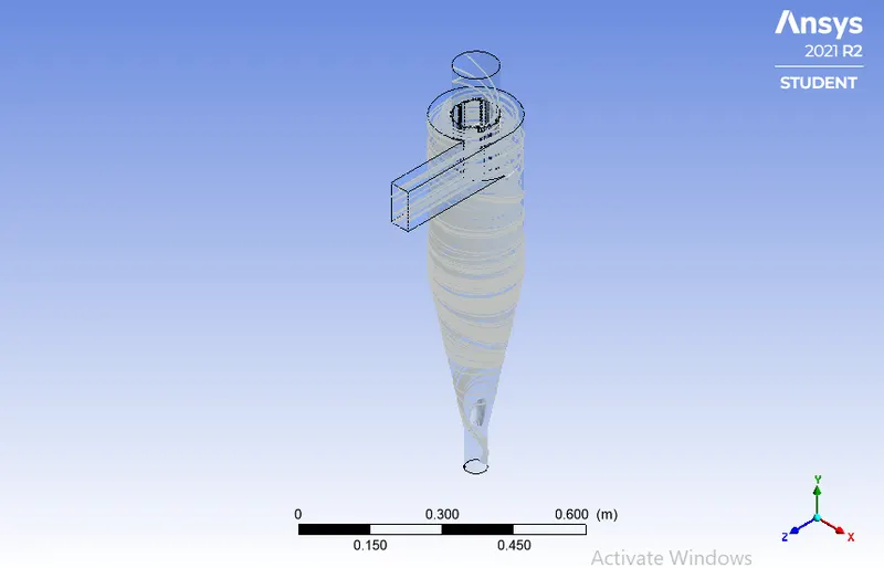
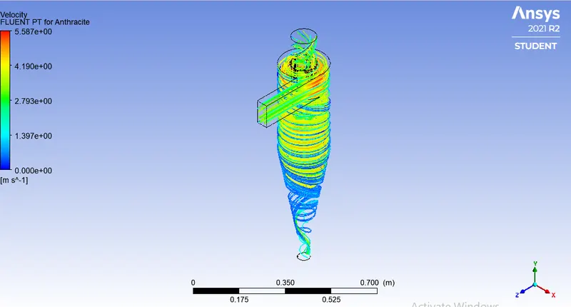
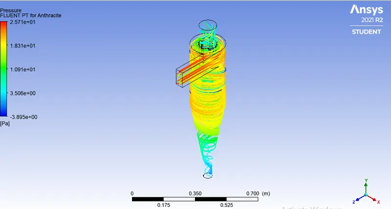
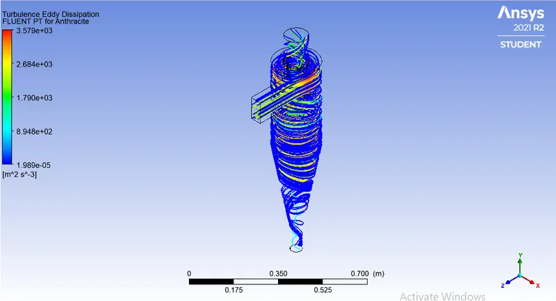
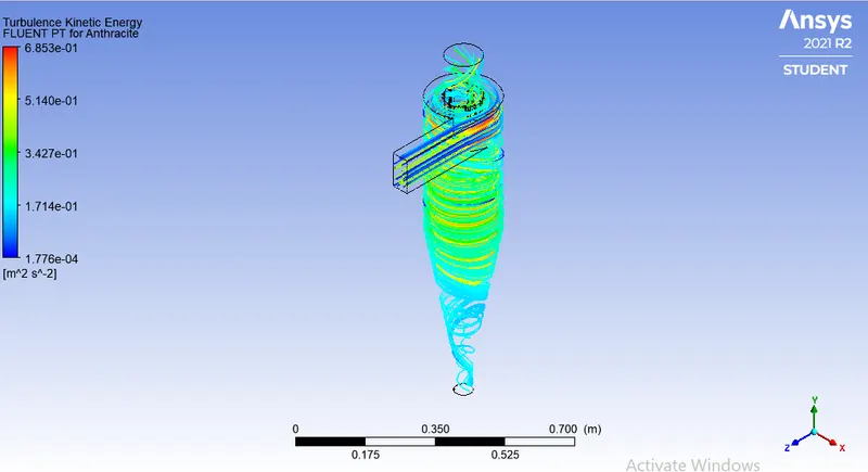
Particle Trajectories

Parametric study:

Input parameter=Particle diameters (1 micrometre to 5 micrometre)

Output parameter= pressures p1, p2

Objective 2(b) : Particle Diameter=2 micrometer, Particle velocity=3m/s

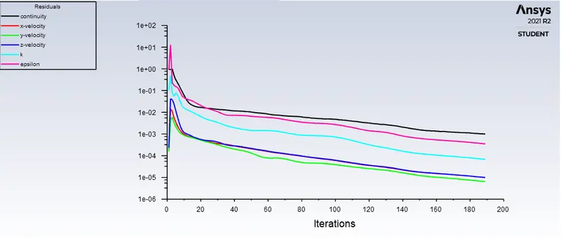
Figure: Scaled Residuals

`eta=251/378=0.66=66%`

Objective 2(c) : Particle Diameter=3 micrometer, Particle velocity=3m/s

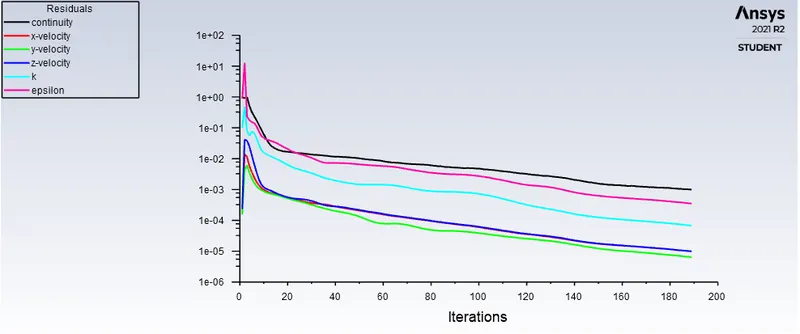
Figure: Scaled Residuals

`eta=269/378=0.71=71%`

Objective 2(d) : Diameter=4 micrometer, velocity=3m/s

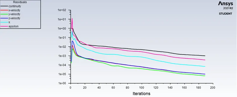
Figure: Scaled Residuals

`eta=306/378=0.80=80%`

Objective 2(e) : Diameter=5 micrometer, velocity=3m/s

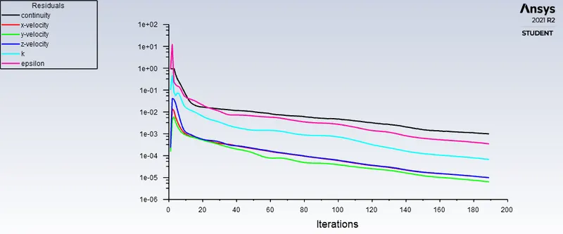
Figure: Scaled Residuals

`eta=310/378=0.82=82%`

Summary

Particle diameter (`mum`)	Particle velocity (m/s)	Tracked particles at inlet	Trapped particles at outlet_bottom	Escaped particles at outlet_top	Incomplete	Separation efficiency(%)
1	3	378	235	142	1	62
2	3	378	251	126	1	66
3	3	378	269	87	22	71
4	3	378	306	72	0	81
5	3	378	310	68	0	82

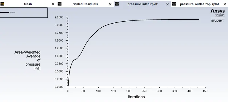
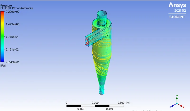
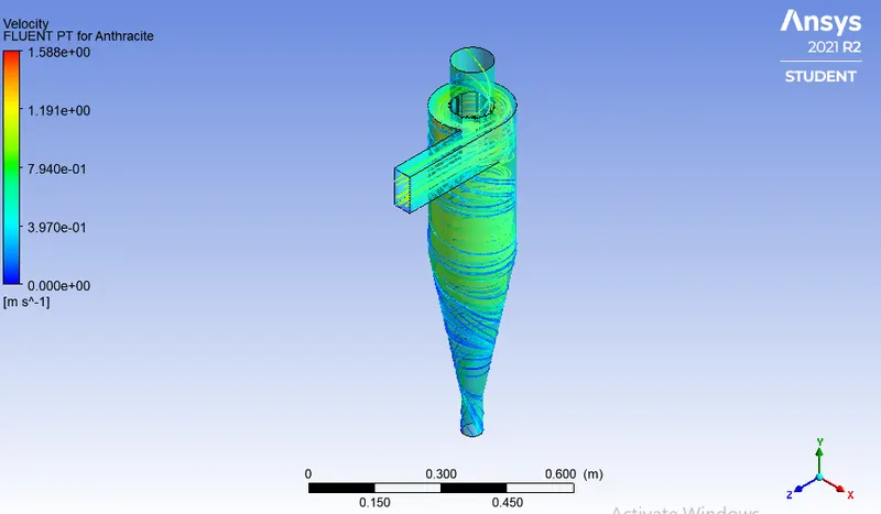
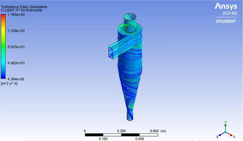
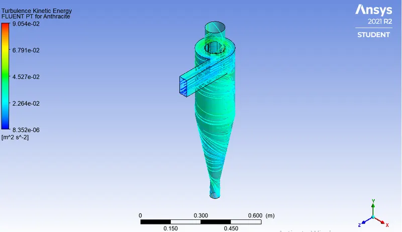
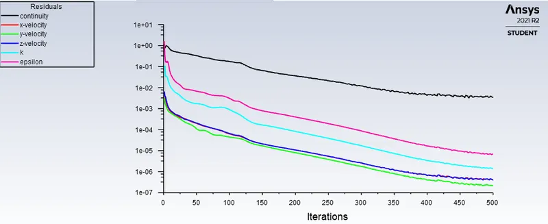
Objective 3(a) : Particle velocity= flow velocity = 1m/s, Particle Diameter=5 micrometer

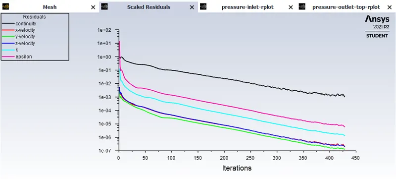
Figure: Scaled Residuals

Particle Trajectories

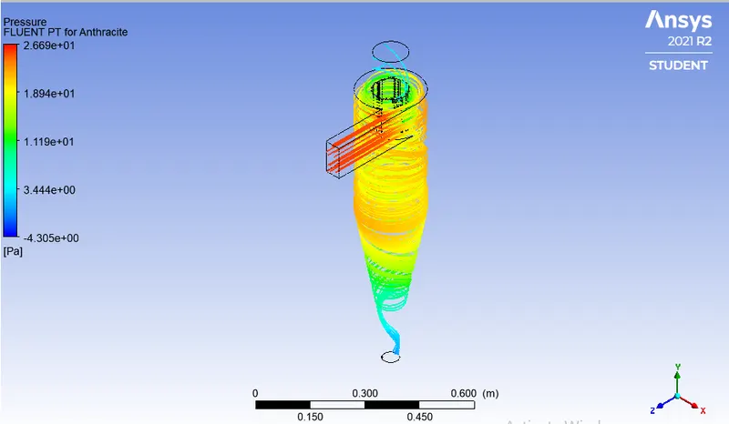
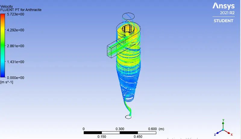
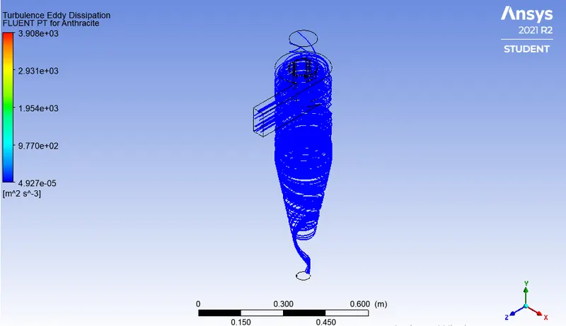
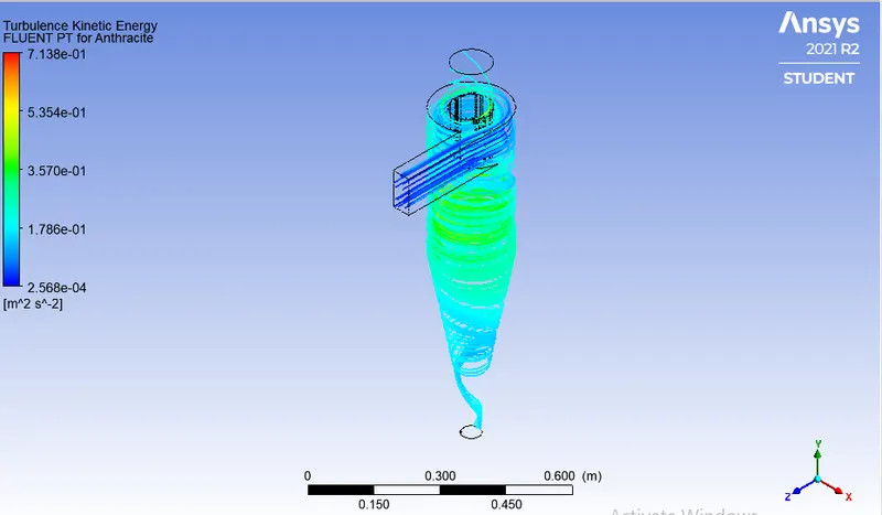
Objective 3(b) : Particle velocity= flow velocity =3m/s, Particle Diameter=5 micrometer

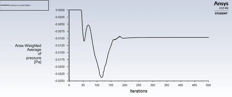
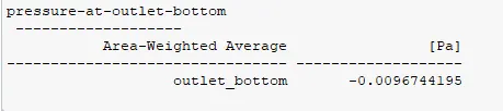
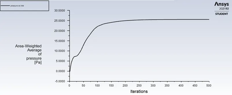
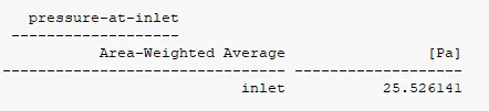
Particle trajectories:

Objective 3(c) : Particle velocity= flow velocity = 5m/s, Particle Diameter=5 micrometer

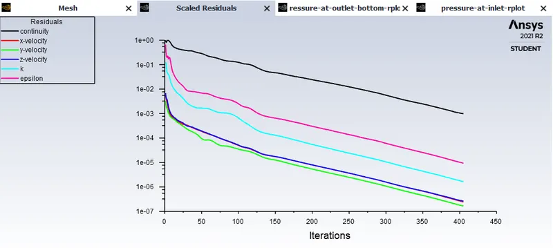
Figure: Scaled Residuals

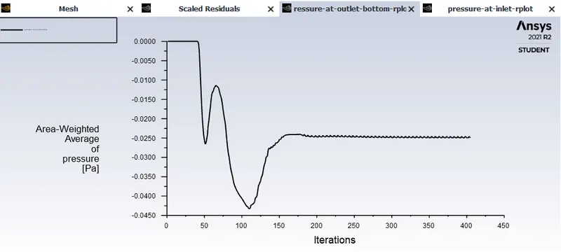
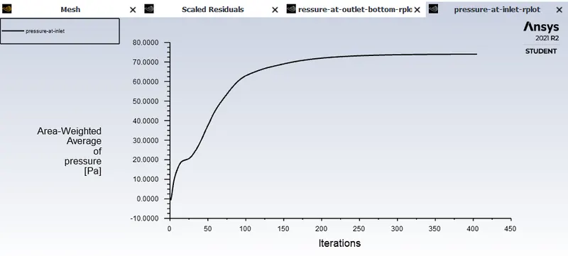
Particle Trajectories

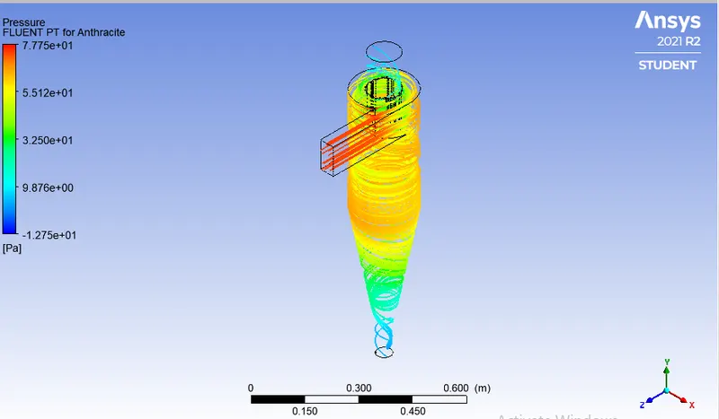
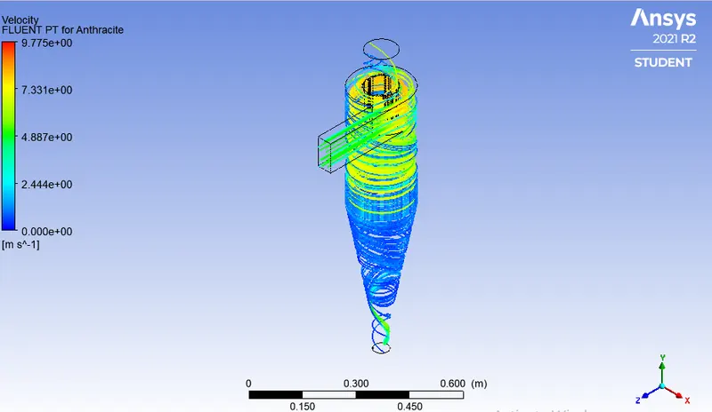
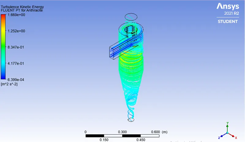
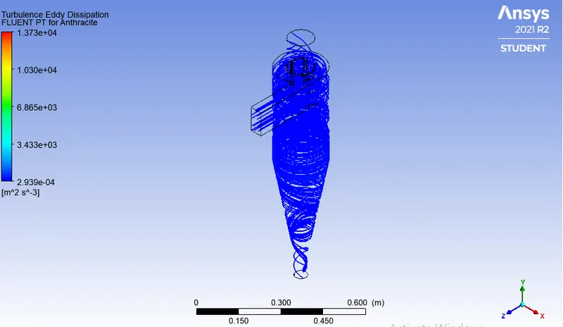
Summary

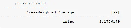
Particle velocity (m/s)	Particle diameter (`mum`)	Tracked particles	Trapped particles at oultlet_bottom	Escaped particles at outlet_top	Separation efficiency (%)	pressure at inlet (Pa)	pressure at Outlet_bottom (Pa)	Pressure drop (Pa)
1	5	378	286	89	75.6	2.1756179	-0.00018427015	2.17580217015
3	5	378	307	70	81.	25.526141	-0.0096744195	25.5358154195
5	5	378	282	60	74.6	73.993843	-0.024897073	74.018740073