Week 7 - Simulation of a 1D Super-sonic nozzle flow simulation using Macormack Method
Main Code

clc; close all; clear all
%% Domain information (Reference:John D.Anderson)
L=3;
nx=31;
x=linspace(0,L,nx)';
dx=x(2)-x(1);
C=0.5; % Courant number
nt=1400;
gamma=1.4;
A=1+2.2*(x-1.5).^2;

[rho1,V1,T1,p1,M1,m1,rho_t1,V_t1,T_t1,p_t1,M_t1,m1_t1,residual1]=non_conservative(x,dx,A,C,nt,gamma);
[rho2,V2,T2,p2,M2,m2,rho_t2,V_t2,p_t2,T_t2,M_t2,m_t2,residual2]=conservative(x,dx,A,C,nt,gamma);
%% Non-conservative plots
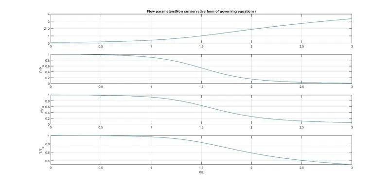
figure(1)
subplot(4,1,1)
plot(x,M1)
grid on
yticks(0:1:5)
ylabel('M')
title('Flow parameters(Non conservative form of governing equations)')
subplot(4,1,2)
plot(x,p1)
grid on
yticks(0:0.2:1)
ylabel('P/P_{o}')
subplot(4,1,3)
plot(x,rho1)
grid on
yticks(0:0.2:1)
ylabel('\rho/\rho_{o}')
subplot(4,1,4)
plot(x,T1)
grid on
yticks(0:0.2:1)
ylabel('T/T_{o}')
xlabel('X/L')

%%  Conservative plots
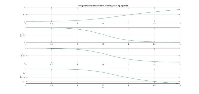
figure(2)
subplot(4,1,1)
plot(x,M2)
grid on
% yticks(0:1:5)
ylabel('M')
title('Flow parameters (conservative form of governing equation')

subplot(4,1,2)
plot(x,p2)
grid on
% yticks(0:0.2:1)
ylabel('P/P_{o}')

subplot(4,1,3)
plot(x,rho2)
grid on
% yticks(0:0.2:1)
ylabel('\rho/\rho_{o}')

subplot(4,1,4)
plot(x,T2)
grid on
% yticks(0:0.2:1)
ylabel('T/T_{o}')
xlabel('x/L')

figure(3)
subplot(4,1,1)
plot(1:nt,rho_t1)
hold on; grid on
plot(1:nt,rho_t2)
ylabel('\rho/\rho_{o}')
legend('Non-conservative','Conservative')
title('Timewise variations of the density, temperature, pressure and mach number at nozzle throat')

subplot(4,1,2)
plot(1:nt,T_t1)
hold on; grid on
plot(1:nt,T_t2)
ylabel('T/T_{o}')
legend('Non-conservative','Conservative')

subplot(4,1,3)
plot(1:nt,p_t1)
hold on; grid on
plot(1:nt,p_t2)
ylabel('p/p_{o}')
legend('Non-conservative','Conservative')

subplot(4,1,4)
plot(1:nt,M_t1)
hold on; grid on
plot(1:nt,M_t2)
ylabel('M')
legend('Non-conservative','Conservative')
xlabel('Number of time steps')

%% Conservative Residual at nozzzle throat i=16
figure(4)
plot(1:nt,residual1)
grid on
xlabel('Number of time steps')
ylabel('Residual')
legend('|(d\rho/dt)|_{av}','|(dv/dt)|_{av}','|(dT/dt)|_{av}')
title('Timewise variation of the absolute values of the time derivatives of nondimensional density, valocity and temperature at the nozzle throat')

%% Non Conservative mass flow
figure(5)
grid on; hold on
plot(x,m1(50,:),'r')
plot(x,m1(100,:),'b')
plot(x,m1(150,:),'g')
plot(x,m1(200,:),'m')
plot(x,m1(700,:),'y')
xticks(0:0.3:3)
legend('50\Deltat','100\Deltat','150\Deltat','200\Deltat','700\Deltat')
xlabel('Non dimensional distance through nozzle (x)')
ylabel('Non dimensional mass flow, (\rhoAV)/(\rho_{o}A_{o}V_{o})')
title('Non dimensional mass flow at six diffetent times during thetime marching approach to the steady state')

%% Conservative mass flow
figure(6)
grid on; hold on
plot(x,m2(100,:),'b')
plot(x,m2(200,:),'m')
plot(x,m2(700,:),'y')
xticks(0:0.3:3)
legend('100\Deltat','200\Deltat','700\Deltat')
xlabel('Non dimensional distance through nozzle (x)')
ylabel('Non dimensional mass flow, (\rhoAV)/(\rho_{o}A_{o}V_{o})')
title('Non dimensional mass flow at six diffetent times during thetime marching approach to the steady state')

%% Steady state mass flow of Conservative and Nonconservative form
figure(7)
grid on; hold on
plot (x,m1(end,:),'r')
plot(x,m2(end,:),'b')
plot(x,0.579*ones(length(x),1),'c')
xlabel('x/L')
ylabel('(\rhoAV)/(\rho_{o}A_{o}V_{o})')
legend('Non-conservative','Conservative','Exact')
title('Steady state mass flow variation')

%% Non-conservative function
function [rho,V,T,p,M,m,rho_t,V_t,T_t,p_t,M_t,m_t,residual]=non_conservative(x,dx,A,C,nt,gamma)
% Initial conditions at t=0
rho=1-0.3146*x;
T=1-0.231*x;
V=(0.1+1.09*x).*T.^0.5;
dt=min(C*(dx./(sqrt(T)+V)));
nx=31;
throat=((nx)+1)/2;
rho_t=zeros(nt,1); m=zeros(nt,length(x));
for k=1:nt
    rho_old=rho; T_old=T; V_old=V;

    %predictor step
    for i=2:length(x)-1
        dVdx_p=(V(i+1)-V(i))/dx;
        dlogA_dx_p=(log(A(i+1))-log(A(i)))/dx;
        drhodx_p=(rho(i+1)-rho(i))/dx;
        dTdx_p=(T(i+1)-T(i))/dx;

        % continuity equation
        drhodt_p(i)=-(rho(i)*dVdx_p)-(rho(i)*V(i)*dlogA_dx_p)-(V(i)*drhodx_p);
        % Momentum equation
        dVdt_p(i)=-V(i)*dVdx_p-(1/gamma)*(dTdx_p+(T(i)/rho(i))*drhodx_p);
        % Energy equation
        dTdt_p(i)=-V(i)*dTdx_p-(gamma-1)*T(i)*(dVdx_p+V(i)*dlogA_dx_p);

        % Intermediate solution update
        rho(i)=rho(i)+(drhodt_p(i)*dt);
        V(i)=V(i)+(dVdt_p(i)*dt);
        T(i)=T(i)+(dTdt_p(i)*dt);
    end

    % corrector loop
    for i=2:length(x)-1
        dVdx_c=(V(i)-V(i-1))/dx;
        dlogA_dx_c=(log(A(i))-log(A(i-1)))/dx;
        drhodx_c=(rho(i)-rho(i-1))/dx;
        dTdx_c=(T(i)-T(i-1))/dx;
        % continuity equation
        drhodt_c(i)=-(rho(i)*dVdx_c)-rho(i)*V(i)*dlogA_dx_c-V(i)*drhodx_c;
        % Momentum equation
        dVdt_c(i)=-(V(i)*dVdx_c)-(1/gamma)*(dTdx_c+(T(i)/rho(i))*drhodx_c);
        % Energy equation
        dTdt_c(i)=-(V(i)*dTdx_c)-(gamma-1)*T(i)*(dVdx_c+V(i)*dlogA_dx_c);
    end

    % average of predictor and corrector
    drhodt=0.5*(drhodt_p+drhodt_c);
    dvdt=0.5*(dVdt_p+dVdt_c);
    dTdt=0.5*(dTdt_p+dTdt_c);

    residual(k,1)=max(abs(drhodt));
    residual(k,2)=max(abs(dvdt));
    residual(k,3)=max(abs(dTdt));

    % Final solution update
    for i=2:length(x)-1
        rho(i)=rho_old(i)+drhodt(i)*dt;
        V(i)=V_old(i)+dvdt(i)*dt;
        T(i)=T_old(i)+dTdt(i)*dt;
    end

    % Boundary condiions
    rho(end)=2*rho(end-1)-rho(end-2);
    V(1)=2*V(2)-V(3);
    V(end)=2*V(end-1)-V(end-2);
    T(end)=2*T(end-1)-T(end-2);
    M=V./sqrt(T);
    p=rho.*T;
    m(k,:)=rho.*A.*V;

    rho_t(k)=rho(throat);
    V_t(k)=V(throat);
    T_t(k)=T(throat);
    p_t(k)=p(throat);
    M_t(k)=M(throat);
    m_t(k)=m(throat);

    rho_exact=0.634*ones(1,1400);
    T_exact=0.833*ones(1,1400);
    p_exact=0.528*ones(1,1400);
    M_exact=1*ones(1,1400);
end
end

%% Function for Conservative form
function [rho,V,T,p,M,m,rho_t,V_t,p_t,T_t,M_t,m_t,residual] = conservative(x,dx,A,C,nt,gamma)
m_t=0.2;
% Initial Conditions
rho_0=zeros(length(x),1);
T_0=rho_0;
V_0=T_0;
for i=1:length(x)
    if x(i)>=0 && x(i)<0.5
        rho_0(i)=1;
        T_0(i)=1;
    elseif x(i)>=0.5 && x(i)<1.5
        rho_0(i)=1-0.366*(x(i)-0.5);
        T_0(i)=1-0.167*(x(i)-0.5);
    elseif x(i)>=1.5 && x(i)<=3
        rho_0(i)=0.634-0.3879*(x(i)-1.5);
        T_0(i)=0.833-0.3507*(x(i)-1.5);
    end
    V_0(i)=0.59/(rho_0(i)*A(i));
end
throat=find(A==1);
rho=rho_0;
T=T_0;
V=V_0;
m=zeros(nt,length(x));
U1=rho.*A;
U2=rho.*A.*V;
U3=rho.*(T./(gamma-1)+0.5*gamma*V.^2).*A;

rho_t=zeros(nt,1);
T_t=rho_t;
V_t=T_t;
p_t=V_t;
M_t=p_t;

residual=zeros(nt,3);
for k=1:nt
    U1_old=U1; U2_old=U2; U3_old=U3;
    dt=min(C*dx./(sqrt(T)+V));
    F1=U2;
    F2=(U2.^2)./U1+((gamma-1)/gamma)*(U3-0.5*gamma*(U2.^2)./U1);
    F3=gamma*U2.*U3./U1-0.5*gamma*(gamma-1)*(U2.^3)./(U1.^2);

    % predictor step
    for i=2:length(x)-1
        dF1dx=(F1(i+1)-F1(i))/dx;
        dF2dx=(F2(i+1)-F2(i))/dx;
        dF3dx=(F3(i+1)-F3(i))/dx;
        dAdx=(A(i+1)-A(i))/dx;
        J2=(1/gamma)*rho(i)*T(i)*dAdx;

        dU1dt_p(i)=-dF1dx;
        dU2dt_p(i)=-dF2dx+J2;
        dU3dt_p(i)=-dF3dx;

        % Intermediate update
        U1(i)=U1(i)+dU1dt_p(i)*dt;
        U2(i)=U2(i)+dU2dt_p(i)*dt;
        U3(i)=U3(i)+dU3dt_p(i)*dt;
    end
    rho=U1./A;
    V=U2./U1;
    T=(gamma-1)*((U3./U1)-0.5*gamma*V.^2);
    F1=U2;
    F2=(U2.^2)./U1+((gamma-1)/gamma)*(U3-0.5*gamma*(U2.^2)./U1);
    F3=gamma*U2.*U3./U1-0.5*gamma*(gamma-1)*(U2.^3)./(U1.^2);

    %corrector step
    for i=2:length(x)-1
        dF1dx=(F1(i)-F1(i-1))/dx;
        dF2dx=(F2(i)-F2(i-1))/dx;
        dF3dx=(F3(i)-F3(i-1))/dx;
        dAdx=(A(i)-A(i-1))/dx;
        J2=(1/gamma)*rho(i)*T(i)*dAdx;

        dU1dt_c(i)=-dF1dx;
        dU2dt_c(i)=-dF2dx+J2;
        dU3dt_c(i)=-dF3dx;
    end

    % Average of predictor and corrector
    dU1dt=0.5*(dU1dt_p + dU1dt_c);
    dU2dt=0.5*(dU2dt_p + dU2dt_c);
    dU3dt=0.5*(dU3dt_p + dU3dt_c);

    residual(k,1)=max(abs(dU1dt));
    residual(k,2)=max(abs(dU2dt));
    residual(k,3)=max(abs(dU3dt));

    % Final solution update
    for i=2:length(x)-1
        U1(i)=U1_old(i) + dU1dt(i)*dt;
        U2(i)=U2_old(i) + dU2dt(i)*dt;
        U3(i)=U3_old(i) + dU3dt(i)*dt;
    end

    % Boundary conditions
    U1(1)=rho(1)*A(1);
    U1(end)=2*U1(end-1)-U1(end-2);
    U2(1)=2*U2(2)-U2(3);
    U2(end)=2*U2(end-1)-U2(end-2);
    U3(1)=U1(1)*((T(1)/(gamma-1))+0.5*gamma*V(1)^2);
    U3(end)=2*U3(end-1)-U3(end-2);
    rho=U1./A;
    V=U2./U1;
    T=(gamma-1)*((U3./U1)-0.5*gamma*V.^2);
    M=V./(T.^0.5);
    p=rho.*T;
    m(k,:)=rho.*A.*V;
    rho_t(k)=rho(throat); V_t(k)=V(throat); T_t(k)=T(throat);
    p_t(k)=p(throat); M_t(k)=M(throat);
end
end

Function code of Non-Conservative form of governing equations
function [rho,V,T,p,M,m,rho_t,V_t,T_t,p_t,M_t,m_t,residual]=non_conservative(x,dx,A,C,nt,gamma)
% Initial conditions at t=0
rho=1-0.3146*x;
T=1-0.231*x;
V=(0.1+1.09*x).*T.^0.5;
dt=min(C*(dx./(sqrt(T)+V)));
nx=31;
throat=((nx)+1)/2;
rho_t=zeros(nt,1); m=zeros(nt,length(x));
for k=1:nt
    rho_old=rho; T_old=T; V_old=V;
    % residual=zeros(nt,3);
    %predictor step
    for i=2:length(x)-1
        dVdx_p=(V(i+1)-V(i))/dx;
        dlogA_dx_p=(log(A(i+1))-log(A(i)))/dx;
        drhodx_p=(rho(i+1)-rho(i))/dx;
        dTdx_p=(T(i+1)-T(i))/dx;

        % continuity equation
        drhodt_p(i)=-(rho(i)*dVdx_p)-(rho(i)*V(i)*dlogA_dx_p)-(V(i)*drhodx_p);
        % Momentum equation
        dVdt_p(i)=-V(i)*dVdx_p-(1/gamma)*(dTdx_p+(T(i)/rho(i))*drhodx_p);
        % Energy equation
        dTdt_p(i)=-V(i)*dTdx_p-(gamma-1)*T(i)*(dVdx_p+V(i)*dlogA_dx_p);

        % Intermediate solution update
        rho(i)=rho(i)+(drhodt_p(i)*dt);
        V(i)=V(i)+(dVdt_p(i)*dt);
        T(i)=T(i)+(dTdt_p(i)*dt);
    end
    % corrector loop
    for i=2:length(x)-1
        dVdx_c=(V(i)-V(i-1))/dx;
        dlogA_dx_c=(log(A(i))-log(A(i-1)))/dx;
        drhodx_c=(rho(i)-rho(i-1))/dx;
        dTdx_c=(T(i)-T(i-1))/dx;
        % continuity equation
        drhodt_c(i)=-(rho(i)*dVdx_c)-rho(i)*V(i)*dlogA_dx_c-V(i)*drhodx_c;
        % Momentum equation
        dVdt_c(i)=-(V(i)*dVdx_c)-(1/gamma)*(dTdx_c+(T(i)/rho(i))*drhodx_c);
        % Energy equation
        dTdt_c(i)=-(V(i)*dTdx_c)-(gamma-1)*T(i)*(dVdx_c+V(i)*dlogA_dx_c);
    end

    % average of predictor and corrector
    drhodt=0.5*(drhodt_p+drhodt_c);
    dvdt=0.5*(dVdt_p+dVdt_c);
    dTdt=0.5*(dTdt_p+dTdt_c);

    residual(k,1)=max(abs(drhodt));
    residual(k,2)=max(abs(dvdt));
    residual(k,3)=max(abs(dTdt));

    % Final solutionupdate
    for i=2:length(x)-1
        rho(i)=rho_old(i)+drhodt(i)*dt;
        V(i)=V_old(i)+dvdt(i)*dt;
        T(i)=T_old(i)+dTdt(i)*dt;

    end
    % Boundary condiions
    rho(end)=2*rho(end-1)-rho(end-2);
    V(1)=2*V(2)-V(3);
    V(end)=2*V(end-1)-V(end-2);
    T(end)=2*T(end-1)-T(end-2);

    M=V./sqrt(T);
    p=rho.*T;
    m(k,:)=rho.*A.*V;

    %% Variables at throat
    rho_t(k)=rho(throat);
    V_t(k)=V(throat);
    T_t(k)=T(throat);
    p_t(k)=p(throat);
    M_t(k)=M(throat);
    m_t(k)=m(throat);

    rho_exact=0.634*ones(1,1400);
    T_exact=0.833*ones(1,1400);
    p_exact=0.528*ones(1,1400);
    M_exact=1*ones(1,1400);


end
end

Function code of Conservative form of governing equations
function [rho,V,T,p,M,m,rho_t,V_t,p_t,T_t,M_t,m_t,residual] = conservative(x,dx,A,C,nt,gamma)
m_t=0.2;
% Initial Conditions
rho_0=zeros(length(x),1);
T_0=rho_0;
V_0=T_0;
for i=1:length(x)
    if x(i)>=0 && x(i)<0.5
        rho_0(i)=1;
        T_0(i)=1;
    elseif x(i)>=0.5 && x(i)<1.5
        rho_0(i)=1-0.366*(x(i)-0.5);
        T_0(i)=1-0.167*(x(i)-0.5);
    elseif x(i)>=1.5 && x(i)<=3
        rho_0(i)=0.634-0.3879*(x(i)-1.5);
        T_0(i)=0.833-0.3507*(x(i)-1.5);
    end
    V_0(i)=0.59/(rho_0(i)*A(i));
end
throat=find(A==1);
rho=rho_0;
T=T_0;
V=V_0;
m=zeros(nt,length(x));
U1=rho.*A;
U2=rho.*A.*V;
U3=rho.*(T./(gamma-1)+0.5*gamma*V.^2).*A;
rho_t=zeros(nt,1);
T_t=rho_t;
V_t=T_t;
p_t=V_t;
M_t=p_t;
residual=zeros(nt,3);
for k=1:nt
    U1_old=U1; U2_old=U2; U3_old=U3;
    dt=min(C*dx./(sqrt(T)+V));
    F1=U2;
    F2=(U2.^2)./U1+((gamma-1)/gamma)*(U3-0.5*gamma*(U2.^2)./U1);
    F3=gamma*U2.*U3./U1-0.5*gamma*(gamma-1)*(U2.^3)./(U1.^2);

    % predictor step
    for i=2:length(x)-1
        dF1dx=(F1(i+1)-F1(i))/dx;
        dF2dx=(F2(i+1)-F2(i))/dx;
        dF3dx=(F3(i+1)-F3(i))/dx;
        dAdx=(A(i+1)-A(i))/dx;
        J2=(1/gamma)*rho(i)*T(i)*dAdx;

        dU1dt_p(i)=-dF1dx;
        dU2dt_p(i)=-dF2dx+J2;
        dU3dt_p(i)=-dF3dx;

        % Intermediate update
        U1(i)=U1(i)+dU1dt_p(i)*dt;
        U2(i)=U2(i)+dU2dt_p(i)*dt;
        U3(i)=U3(i)+dU3dt_p(i)*dt;
    end
    rho=U1./A;
    V=U2./U1;
    T=(gamma-1)*((U3./U1)-0.5*gamma*V.^2);
    F1=U2;
    F2=(U2.^2)./U1+((gamma-1)/gamma)*(U3-0.5*gamma*(U2.^2)./U1);
    F3=gamma*U2.*U3./U1-0.5*gamma*(gamma-1)*(U2.^3)./(U1.^2);

    %corrector step
    for i=2:length(x)-1
        dF1dx=(F1(i)-F1(i-1))/dx;
        dF2dx=(F2(i)-F2(i-1))/dx;
        dF3dx=(F3(i)-F3(i-1))/dx;
        dAdx=(A(i)-A(i-1))/dx;
        J2=(1/gamma)*rho(i)*T(i)*dAdx;

        dU1dt_c(i)=-dF1dx;
        dU2dt_c(i)=-dF2dx+J2;
        dU3dt_c(i)=-dF3dx;
    end

    % Average of predictor and corrector
    dU1dt=0.5*(dU1dt_p + dU1dt_c);
    dU2dt=0.5*(dU2dt_p + dU2dt_c);
    dU3dt=0.5*(dU3dt_p + dU3dt_c);

    residual(k,1)=max(abs(dU1dt));
    residual(k,2)=max(abs(dU2dt));
    residual(k,3)=max(abs(dU3dt));

    % Final solution update
    for i=2:length(x)-1
        U1(i)=U1_old(i) + dU1dt(i)*dt;
        U2(i)=U2_old(i) + dU2dt(i)*dt;
        U3(i)=U3_old(i) + dU3dt(i)*dt;
    end

    % Boundary conditions
    U1(1)=rho(1)*A(1);
    U1(end)=2*U1(end-1)-U1(end-2);
    U2(1)=2*U2(2)-U2(3);
    U2(end)=2*U2(end-1)-U2(end-2);
    U3(1)=U1(1)*((T(1)/(gamma-1))+0.5*gamma*V(1)^2);
    U3(end)=2*U3(end-1)-U3(end-2);
    rho=U1./A;
    V=U2./U1;
    T=(gamma-1)*((U3./U1)-0.5*gamma*V.^2);
    M=V./(T.^0.5);
    p=rho.*T;
    m(k,:)=rho.*A.*V;

    %% Variables at throat
    rho_t(k)=rho(throat);
    V_t(k)=V(throat);
    T_t(k)=T(throat);
    p_t(k)=p(throat);
    M_t(k)=M(throat);
    m_t(k)=m(throat);
end
end
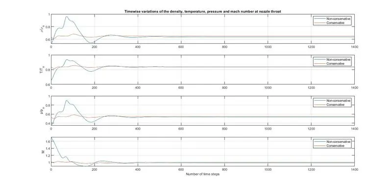
The above figure shows that up to a certain number of time steps, there are fluctuations in the non-conservative form of governing equations. it means the non-conservative form gives an unstable result till approximate 500-time steps. then after it becomes stable. beyond 500 time steps, there is no difference in conservative and nonconservative form.
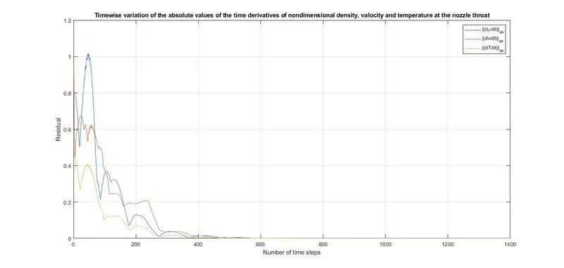
at early times, time derivatives are large and they oscillate in value. these oscillations are associated with various unsteady compression and expansion waves which propagate through the nozzle during the transient process.
At later times, the time derivatives rapidly grow small. theoretically, the required time to reach a steady-state is infinite. but in the above figure, the steady-state condition reached in a finite number of time steps(700-time steps). this seems the characteristics of the MacCormack Technique.
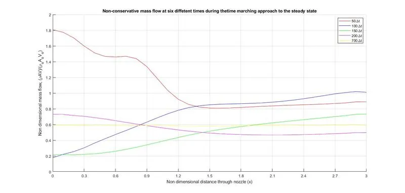
after 200 time steps, the mass flow distribution is beginning to settle down. and after700-time step mass flow rate remains constant throughout the nozzle means rho*A*V=constant. this says that the mass flow rate has converged to a constant, steady-state value throughout the nozzle.
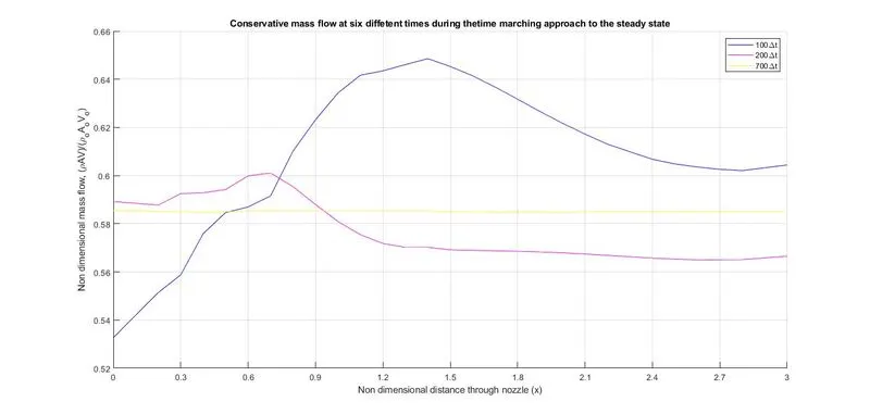
the result at 100-time steps shows a somewhat humped distribution. and at the 200-time step, mass flow distribution is becoming more constant. and at 700-time steps, dimensionless mass flow rate becomes a constant value and quite close to the exact analytical value of 0.579.
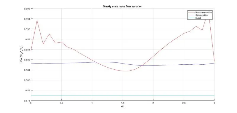
in the above figure, the nonconservative mass flow has an oscillation at both inflow and outflow boundaries. whereas conservative mass flow has a constant value.
Grid Independence: solving a problem by using CFD, we generally discretize the domain in a finite number of grid points. assume there are N gridpoints. and if everything goes well during simulation, then it will give qualitative values of flow field variables at these N grid points. if we increase the grid points let's say 2N (means decreasing grid size) if there is a significant difference in flow field variables then we can say that our solution is a function of the number of grid points. otherwise, it will be grid independence.
in a given challenge we used N=31 grid points. now we double it 2N=62
| Conditions at the nozzle throat | |||||
| `rho/(rho_o)` | `T/(T_o)` | `p/(p_o)` | M | ||
| Non-conservative | N=31 | 0.6387 | 0.8365 | 0.5342 | 0.9994 |
| N=62 | 0.6377 | 0.8354 | 0.5327 | 0.9998 | |
| Exact analytical solution | 0.634 | 0.833 | 0.528 | 1.000 | |
| Conservative | N=31 | 0.6504 | 0.7831 | 05464 | 0.9817 |
| N=62 | 0.6382 | 0.8352 | 0.5330 | 0.9993 | |
| Exact analytical solution | 0.634 | 0.833 | 0.528 | 1.000 | |
| Courant Number | `rho/(rho_o)` | `T/(T_o)` | `p/(p_o)` | M |
| 0.5 | 0.6387 | 0.8365 | 0.5342 | 0.9994 |
| 0.7 | 0.6391 | 0.8366 | 0.5408 | 0.9992 |
| 0.9 | 0.6395 | 0.8368 | 0.5351 | 0.9989 |
| 1.0 | 0.6397 | 0.8368 | 0.5353 | 0.9988 |
| 1.1 | 0.6399 | 0.8369 | 0.5355 | 0.9987 |
| 1.2 | the program went unstable and blew up | |||
| Exact analytical solution | 0.634 | 0.833 | 0.528 | |
Summary of Non-conservative and Conservative form of governing equations:
1. from figure 7 conservative form yields a better mass flow distribution. the conservation form simply does a better job of conserving mass.
2. From figure 4 nonconservative form leads to a smaller residual. the quality of the numerical algorithm is represented by the amount by which the residual decay. in this sense, nonconservative does a better job.
3. the non-conservative form seems to produce slightly more accurate results for the primitive variables. whereas conservative form seems to produce slightly more accurate results for the flux variables.
4. solution of the conservative form requires more work. because we need to decode the primitive variables from flux variables. whereas nonconservative form does not required decoding.