Week 8 - Simulating Cyclone separator with Discrete Phase Modelling
Aim:- To perform analysis on a cyclone separator and calculate the separation efficiency and pressure drop.
Objective:-
- To write a few words about any four empirical models used to calculate the cyclone separator efficiency.
- To perform an analysis on a given cyclone separator model by varying the particle diameter from 1 μm to 5 μm and calculate the separation efficiency in each case.
- To perform an analysis on a given cyclone separator model by varying the particle velocity from 1 m/sec to 5 m/sec and calculate the separation efficiency and pressure drop in each case.
Boundary Conditions:-
Inlet and wall:- Reflect
Outlet(Top):- Escape
Outlet(Bottom/dustbin) - Trap
1)Theory:
Cyclone collection efficiency (`eta`), is defined as the fraction of particles of a given size that is retained by the cyclone.
The theories that have been developed to predict efficiency differ greatly in complexity. There is a general agreement that operating parameters of the system should be used to predict performance, and most theories account for the influence of particle diameter and density, and gas velocity and viscosity.
There is less agreement on the effects of cyclone dimensions and geometry. Some theories consider all eight cyclone dimensions while others include as few as three.
Separation of particles in the cyclone is due to the centrifugal force caused by the spinning gas stream; this force throws particles outward to the cyclone wall. Opposing this outward particle motion is an inward drag force caused by gas flowing toward the axis of the cyclone prior to discharge. All efficiency theories set up a balance between these opposing forces. By making different assumptions about gas flow through the cyclone, various terms in the force balance can be dismissed as insignificant. Since the relative importance of these terms will change with cyclone design and operating conditions, it is unlikely that any single set of assumptions will predict cyclone efficiency accurately for all applications. Leith (1979) has identified three general approaches to predicting cyclone collection efficiency as discussed below.[1]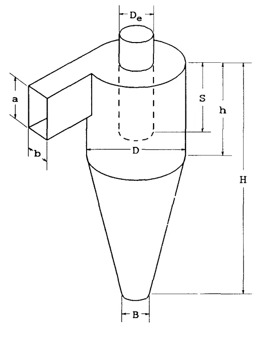
Critical Diameter: Timed Flight Approach
This method assumes that particles enter the cyclone a certain radial distance from the cyclone axis. Particles must travel outward from this position to the wall to be collected; the critical particle is the size that travels exactly this distance during its residence time in the cyclone. Different assumptions about initial radial position and residence time lead to different approximate solutions.
i) Lapple Method:
Lapple model was developed based on force balance without considering the flow resistance. Lapple assumed that a particle entering the cyclone is evenly distributed across the inlet opening. The particle that travels from inlet half width to the wall in the cyclone is collected with 50% efficiency. The semi empirical relationship developed by Lapple to calculate a 50% cut diameter [1][2], `d_(pc)`, is
`d_(pc) = [ frac{9 mu_g b} {2 pi N_e v_i (rho_p - rho_g)}]^(1/2)`
where
`mu_g` is the dynamic viscosity of gas,
`rho_g` is the density of gas,
`rho_p` is the density of particles,
`v_i` is the inlet velocity,
`N_e` is the number of revolutions, is given as follows
`N_e = frac{1}{a} *[ h - frac{H -h}{2}]`
The efficiency of collection of any size of particle is given by `eta_i`,
`eta_i = frac{1}{1+(frac{d_(pc)}{bar(d)_("pi")})^2}`
where
`bar(d)_("pi")` is an average particle size.
Critical Diameter: Static Particle Approach
The static particle approach determines the particle diameter for which centrifugal force is exactly balanced by the drag force. These particles should rotate indefinitely around the edge of the core, the central region of the cyclone below the gas outlet. Drag force on smaller particles exceeds centrifugal force so they are carried inward and out of the cyclone. Larger particles spin out toward the cyclone wall and are collected. The static particle approach predicts a sharp increase in cyclone efficiency from zero for particles smaller than the critical diameter to unity for larger particles.
In practice, a sharp separation is never observed because of fluctuations in radial and tangential gas velocities over the height of the cyclone, and the efficiency for the critically sized particle is often assumed to be 50%.
ii) Barth Model:
Barth's (1956) efficiency theory, widely cited in European literature, is an example of the static particle approach. He defined the cyclone core as the imaginary cylindrical extension of the gas outlet down to the cyclone bottom or cone wall. Barth calculated the terminal settling velocity for the static particle as `v_(ts)^**` [1],
`v_(ts)^** = frac{Q g}{2 pi h^** v_(t)^2}`
where
`Q`is volumetric flowrate,
`g`is acceleration due to gravity
The collection efficiency for any other par- ticle size is determined from the ratio of its settling velocity to `v_(ts)^**`,
`frac{v_(ts)}{v_(ts)^**} = frac{ pi h^** v_(t)^2 rho_p d^2}{9 mu_g Q}`
where,the height of the cyclone core is `h^**`,
`h^** = H - S ` if `D_e <= B`
`h^** = frac{(H - h) (D - D_e)}{(D - B)} + (h - S) ` if `D_e > B`
Barth calculated the tangential gas velocity (`v_t`) at the edge of the cyclone core as
`v_t = v_o [frac{(D_e /2) (D-b) pi}{2 a b alpha + h^** (D-b) lamda pi}]`
where
`v_o`is outlet velocity,
`lamda` is a friction factor that Barth assumed to be 0.02 and
`alpha = 1 - 1.2(b/D)`.
Barth's plot of efficiency versus the ratio `v_(ts)^** / v_(ts)`; it is based on experimental results for several cyclone designs. Barth's curve is closely approximated by
`eta_i = frac{1}{1+(frac{v_(ts)^**}{v_(ts)})^3.2}`
Fractional Efficiency Approach
Recent cyclone theories allow direct calculation of collection efficiency for particles of any size by cyclones of any design. The entire fractional efficiency curve can be determined without resorting to a generalized efficiency curve based on a critical diameter.
Examples of this approach are the Leith-Licht (1972) theory and a newer the- ory by Dietz (1981).[1]
iii) Leith-Licht (1972) Model
Gas flow in industrial-sized cyclones is always turbulent. The Leith-Licht model accounts for turbulence by assuming that at any height in the cyclone, uncollected dust is completely and uniformly mixed. An average residence time in the cyclone is determined from cyclone dimensions and gas throughput.
The resultant expression for collection efficiency is
`eta_i = 1 - exp[-2 (C Psi)^(frac{0.5}{n+1})]`
The influences of particle and gas properties are combined in `Psi`, a modified inertia parameter
`Psi = frac{ rho_p d^2 v_i (n+1)}{18 mu_g D}`
The term C is a dimensionless geometry parameter that depends only on the eight cyclone dimension ratios. C is constant for any cyclone design, and each design has a unique value of C.
`C = frac{pi D^2}{a b} [2{1-(frac{D_e}{D})^2} (frac{S}{D}-frac{a}{2D}) + frac{1}{3} (frac{S+l-h}{D}) (1+ frac{d_c}{D} + frac{d_c^2}{D^2}) + frac{h}{D} -(frac{D_e}{D})^2 frac{l}{D} - frac{S}{D}]`
The natural length of the cyclone`l`, was defined by Alexander (1949) as the farthest distance the spinning gas extends below the gas outlet duct.
`l =2.3 D_e (frac{D^2}{a b})^(1/3)`
The cone diameter `d_c` at the natural length `l` is,
`d_c = D - frac{(D-B)(S+l-h)}{(H-h)}`
If the natural length`l` exceeds `(H - S)`, then `l` in Equations for `d_c` and `C` is replaced by `(H - S)`.
The vortex exponent `n`, describes the change in tangential gas velocity with radial position, `r`, in the cyclone i.e. `v_t r^n = "constant"`. Experimental studies of cyclone flow patterns have measured `n` in the range of 0.5 to 0.9. Alexander (1949) presented an empirical expression to calculate `n` for any cyclone diameter and gas temperature.
`n = 1 - [(1 - 0.67 D^0.14)(T/283)^0.3]` .
iv) The Dietz (1981) model
The Dietz (1981) model represents a refinement of the Leith-Licht method. The model divides the cyclone into three regions: the entrance region (the annular space around the outlet duct at the top of the cyclone); the downflow region (corresponding to the vortex below the level of the outlet duct); and the core region (formed by the extension of the outlet duct to the bottom of the cyclone). Turbulence is assumed to produce a uniform radial concentration profile for uncollected particles with each region. To approximate a distribution of particle residence times in the cyclone, the theory allows for the exchange of particles between the downflow and core regions.
The Dietz model calculates cyclone collection efficiency as
`eta_i = 1 - [K_0 - (K_1^2 + K_2)^0.5](exp[frac{- pi (2S-a) rho_p d^2 v_i}{18 mu_g a b}])`
The subscripted `K` terms are functions of particle and gas properties as well as cyclone dimensions.
`K_0 = frac{1}{2} [1+(frac{D_e}{D})^(2n) (1+frac{9 mu_g a b}{pi rho_p l d^2 v_i})]`
`K_1 = frac{1}{2} [1-(frac{D_e}{D})^(2n) (1+frac{9 mu_g a b}{pi rho_p l d^2 v_i})]`
`K_2 = (frac{D_e}{D})^(2n)`
As in the Leith-Licht theory, `l` should be replaced by `(H - S)` if the natural length `l` exceeds `(H - S)` and the vortex exponent `n` can be calculated as defined earlier.
Overall Separation efficiency(`eta`):
Overall Separation efficiency for cyclone separator is given as the ratio of mass flow rate of particles collected (seperated) to the mass flow rate fed at the inlet. i.e.
`eta = frac{M_c}{M_f} = frac{(M_f - M_e)}{M_f}= 1- frac{M_e}{M_f}`
as `M_f = M_c + M_e` is the mass balance equation for a cyclone separator.
where
`M_f ` is mass flow rate of particles at inlet ,
`M_e` is mass flow rate of escaped particles at top outlet and
`M_c` is the mass flow rate of collected particles at the bottom outlet.
Case Setup:
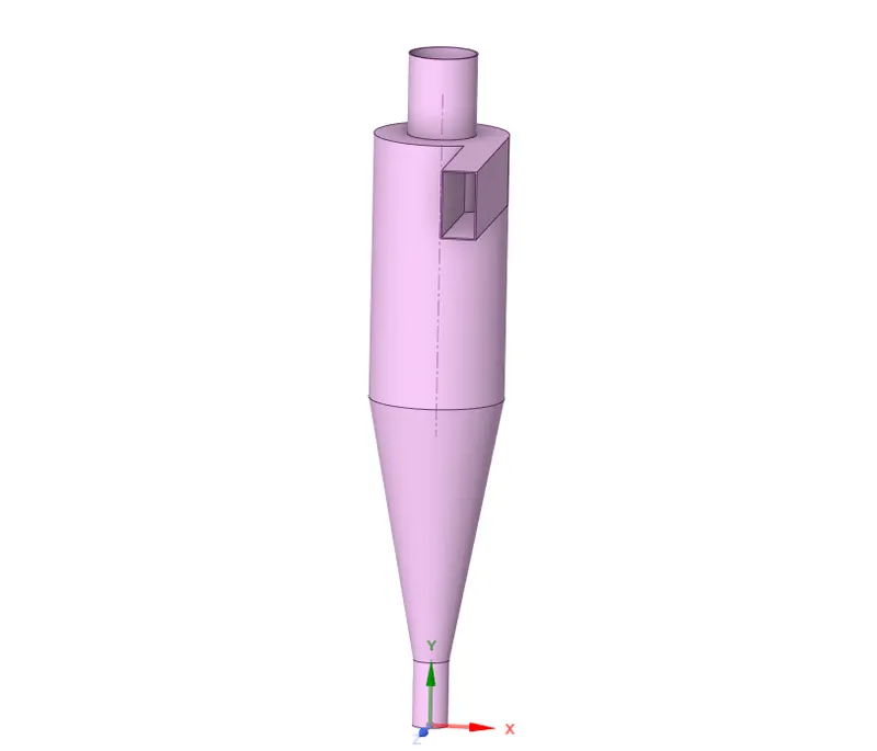
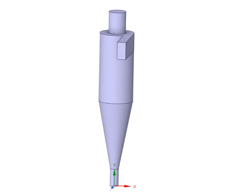
Geometry: The volume has been extracted from the given geometry with the help of volume extraction utility inside the spaceclaim. The physical geometrical model has been suppressed for physics.
| Cyclone Separator Geometry | Cyclone Separator Extracted volume | |||
 |
 |
|||
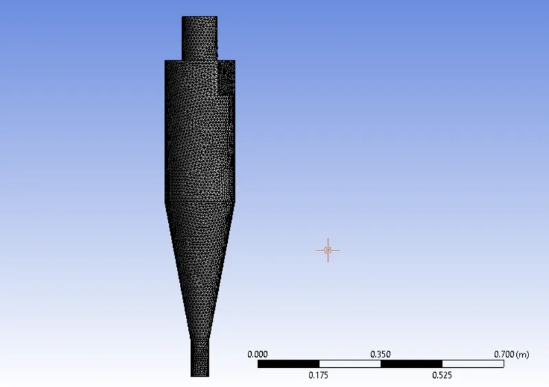
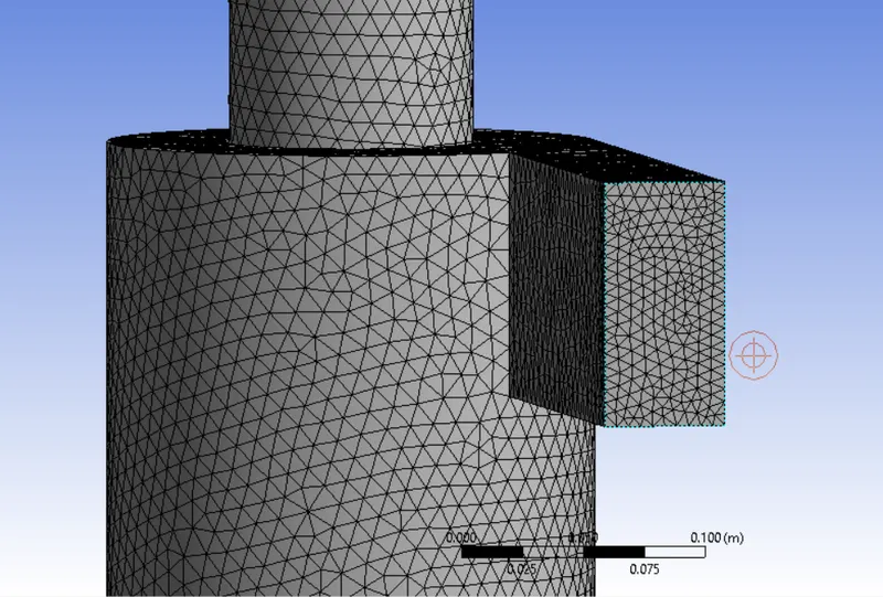
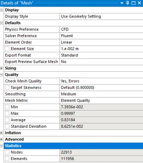
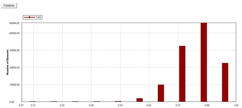
Meshing: The extracted volume of the cyclone separator has been meshed inside the ansys meshing tool and parts have been named using named selection. The inlet face has been meshed finer using mesh sizing method , to increase the number particles to be injected from inlet.
| Mesh | Mesh at inlet face | |||
 |
 |
|||
| Mesh Details | Mesh Metrics | |||
 |
 |
Fluent Setup:
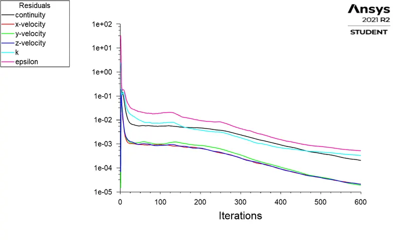
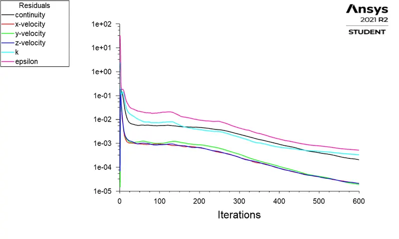
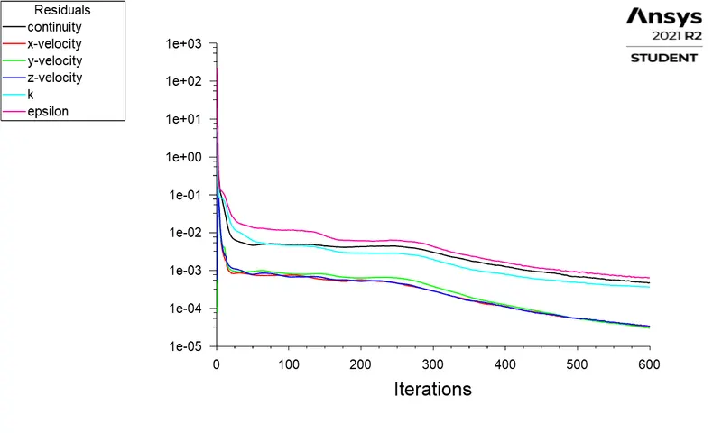
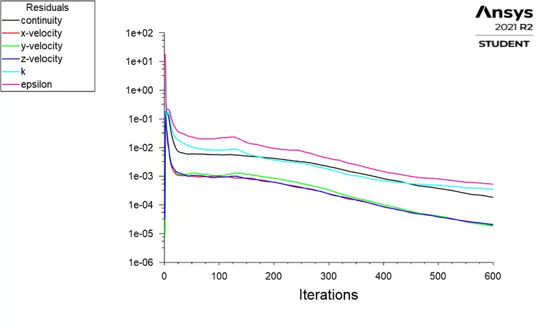
Pressure based steady state solver using SIMPLE algorithm has been to simulate the cyclone separator. The RNG k-epsilon turbulence model with swirl dominated flow and standard wall function is used with second order accuracy for k and epsilon. The coupled Discrete Phase Model has been set for injection of anthracite inert particles with necessary details. Cell zone and boundary conditions are set as required. Standard initialisation has been done with the input data from the inlet and simulation has been done for 600 number of iterations. The particles track data file is exported and saved along with Case and data files.
Post Processing: The results have been post processed in the CFD Post by importing the particle data file. The Results are analysed.
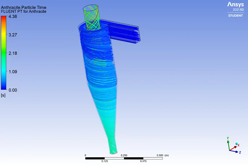
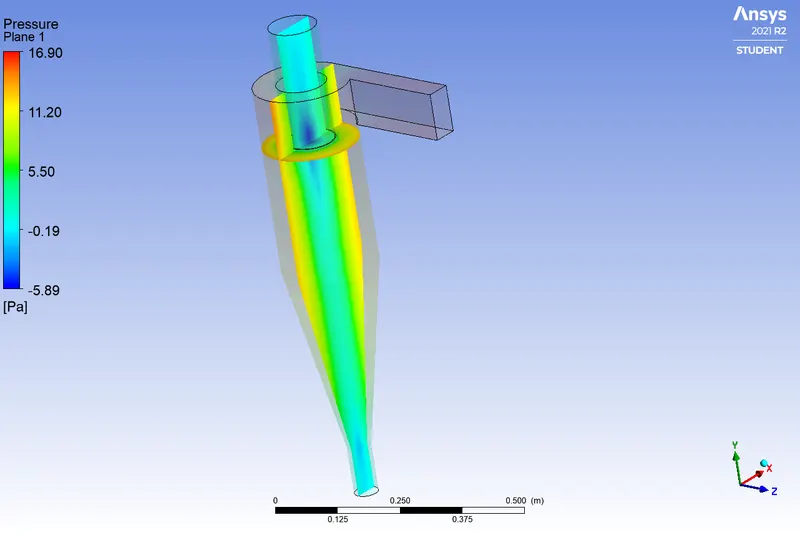
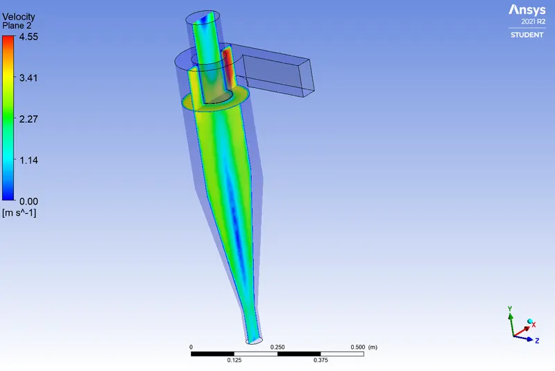
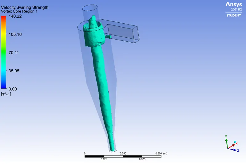
2)Analysis of Cyclone Separator performance with varying particle diameter from 1 `mu m` to 5 `mu m` (Particle and Gas Velocity`3 m/s`).
i) Case I: 1 `mu m` Particle diameter with 3 `m/s` particle and gas velocity.
| 1) | Residuals Graph | 2) | Particle residence time | |
 |
 |
|||
| 3) | Pressure contours on sectional planes | 4) | Velocity contours on sectional planes | |
 |
 |
|||
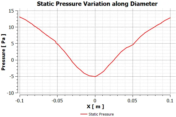
| 5) | Vortex core with strength of level 0.35 ( 49.08 `s^-1`) | 6) | Pressure variation along diameter just below the outlet | |
 |
 |
|||
| 7) | Particle Track Results | 8) | Pressure drop Results | |
| `m_f` = 400 ; `m_e`= 69 ; `m_c`= 331. Thus, Overall Separation Efficiency `eta = frac{331}{400} = 0.8275 = 82.75%`. |
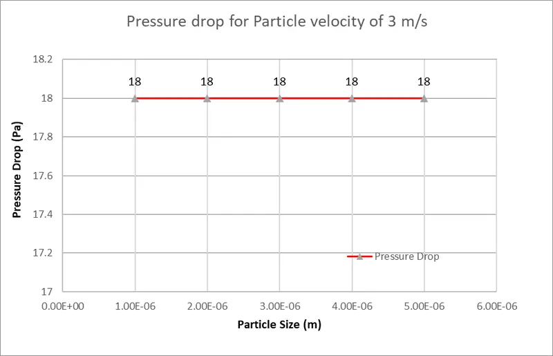
Max `Delta P` = `16.90 - (-5.89)`= `21.79` Pa; `Delta P` across diameter =`13 - (-5)`= `18` Pa. |
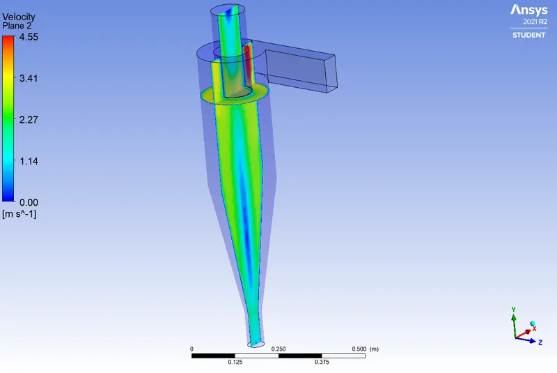
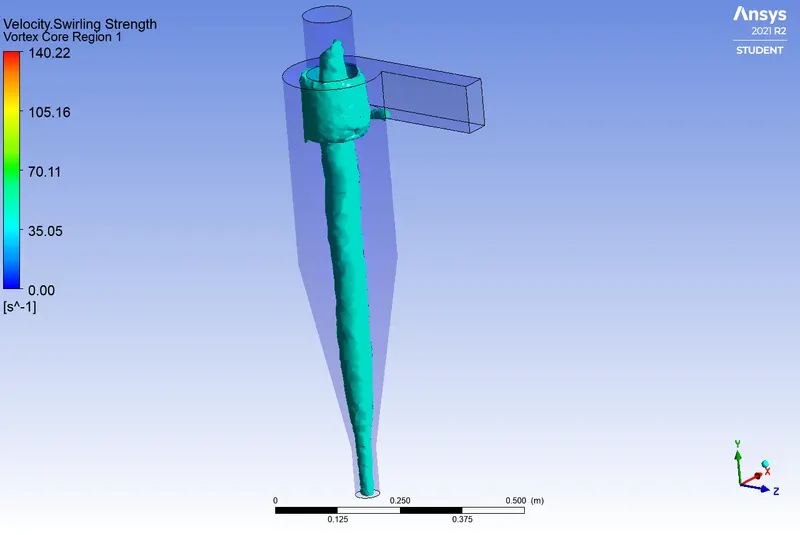
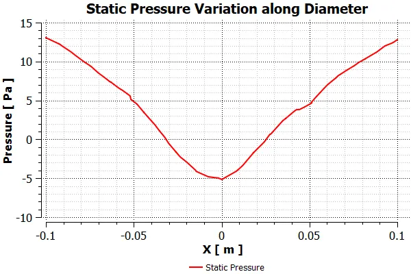
ii) Case II: 2 `mu m` Particle diameter with 3 `m/s` particle and gas velocity.
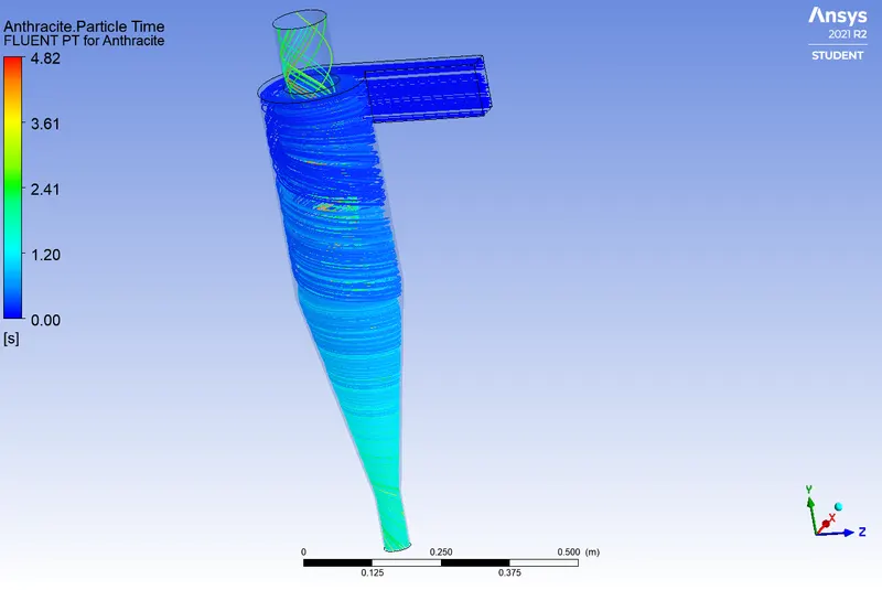
| 1) | Residuals Graph | 2) | Particle residence time | |
 |
 |
|||
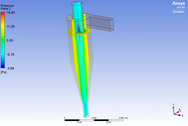
| 3) | Pressure contours on sectional planes | 4) | Velocity contours on sectional planes | |
 |
 |
|||
| 5) | Vortex core with strength of level 0.35 ( 49.08 `s^-1`) | 6) | Pressure variation along diameter just below the outlet | |
 |
 |
|||
| 7) | Particle Track Results | 8) | Pressure drop Results | |
| `m_f` = 400 ; `m_e`= 47 ; `m_c`= 353. Thus, Overall Separation Efficiency `eta = frac{353}{400} = 0.8825 = 88.25%`. |
Max `Delta P` = `16.90 - (-5.89)`= `21.79` Pa; `Delta P` across diameter =`13 - (-5)`= `18` Pa. |
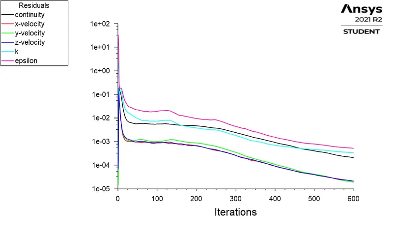
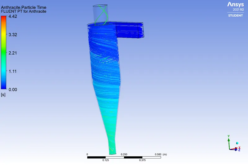
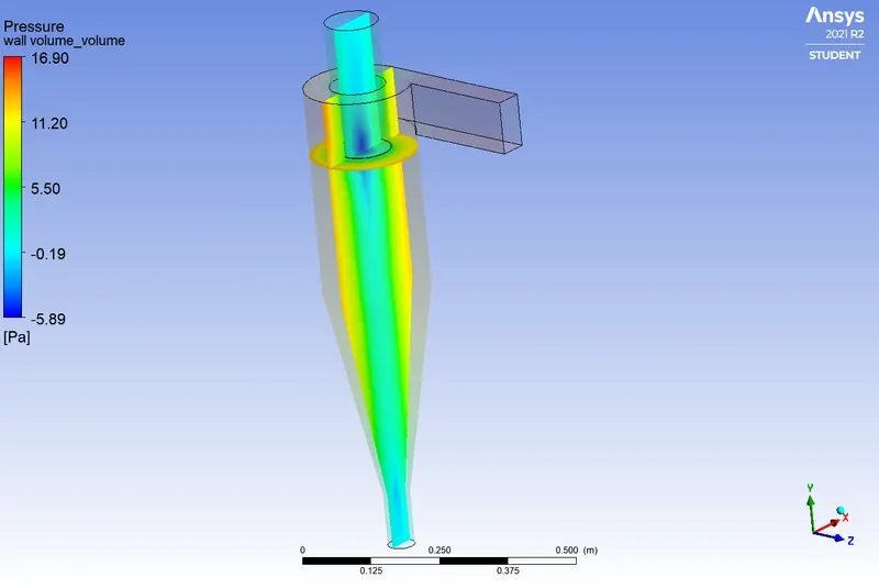
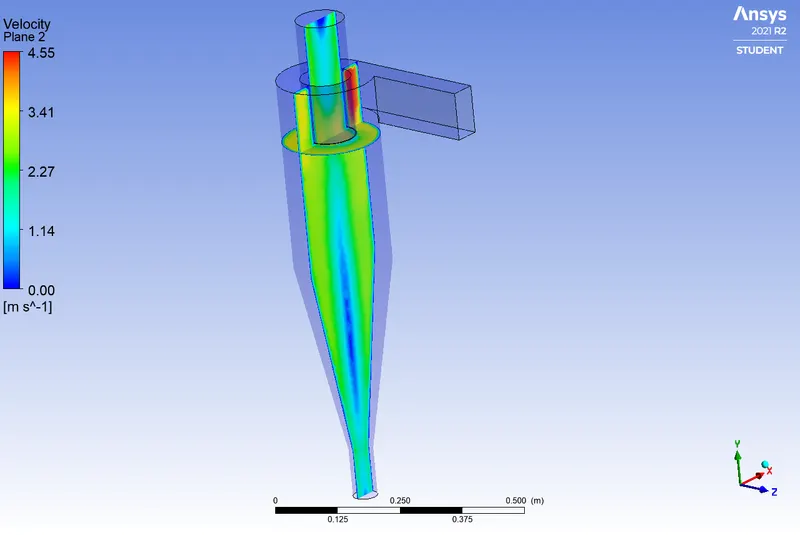
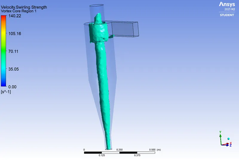
iii) Case III: 3 `mu m` Particle diameter with 3 `m/s` particle and gas velocity.
| 1) | Residuals Graph | 2) | Particle residence time | |
 |
 |
|||
| 3) | Pressure contours on sectional planes | 4) | Velocity contours on sectional planes | |
 |
 |
|||
| 5) | Vortex core with strength of level 0.35 ( 49.08 `s^-1`) | 6) | Pressure variation along diameter just below the outlet | |
 |
|
|||
| 7) | Particle Track Results | 8) | Pressure drop Results | |
| `m_f` = 400 ; `m_e`= 15 ; `m_c`= 385. Thus, Overall Separation Efficiency `eta = frac{385}{400} = 0.9625 = 96.25%`. |
Max `Delta P` = `16.90 - (-5.89)`= `21.79` Pa; `Delta P` across diameter =`13 - (-5)`= `18` Pa. |
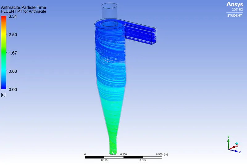
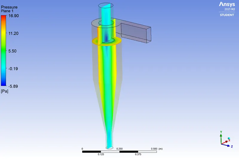
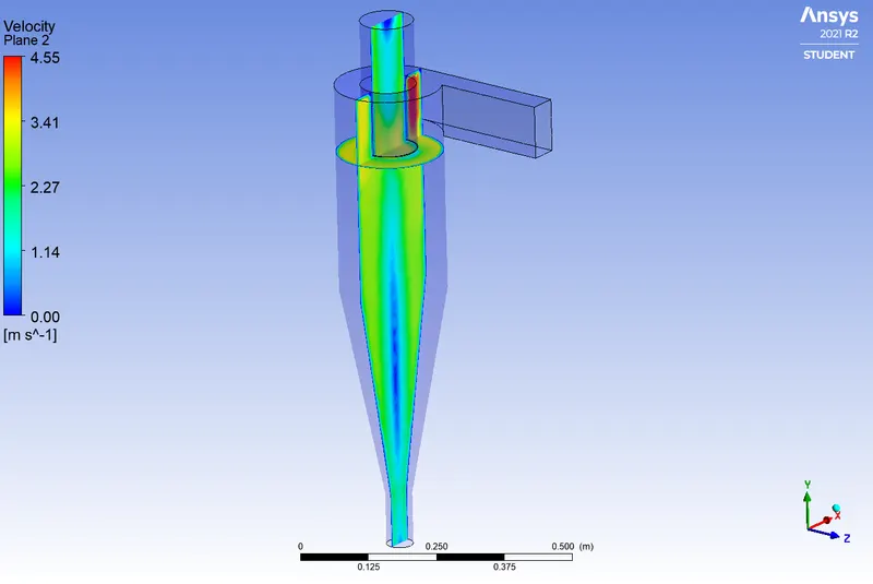
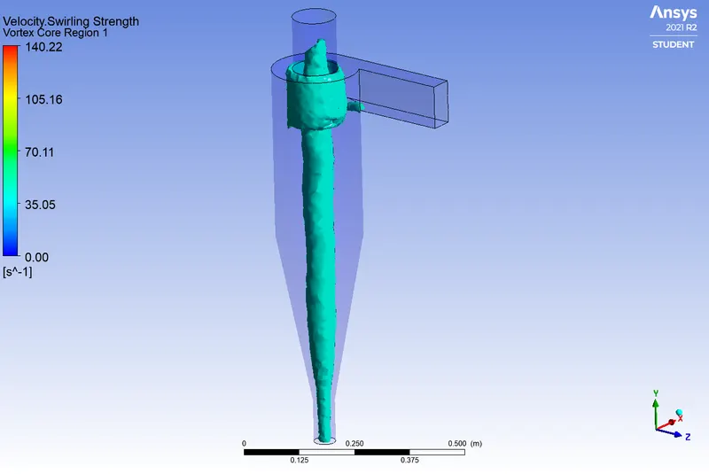
iv) Case IV: 4 `mu m` Particle diameter with 3 `m/s` particle and gas velocity.
| 1) | Residuals Graph | 2) | Particle residence time | |
|
 |
|||
| 3) | Pressure contours on sectional planes | 4) | Velocity contours on sectional planes | |
 |
 |
|||
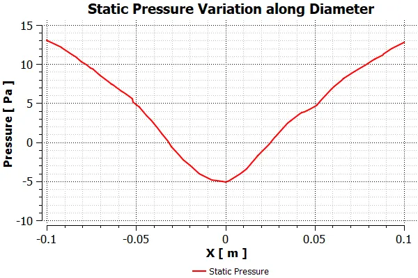
| 5) | Vortex core with strength of level 0.35 ( 49.08 `s^-1`) | 6) | Pressure variation along diameter just below the outlet | |
 |
 |
|||
| 7) | Particle Track Results | 8) | Pressure drop Results | |
| `m_f` = 400 ; `m_e`= 5 ; `m_c`= 395. Thus, Overall Separation Efficiency `eta = frac{395}{400} = 0.9875 = 98.75%`. |
Max `Delta P` = `16.90 - (-5.89)`= `21.79` Pa; `Delta P` across diameter =`13 - (-5)`= `18` Pa. |
v) Case V: 5 `mu m` Particle diameter with 3 `m/s` particle and gas velocity.
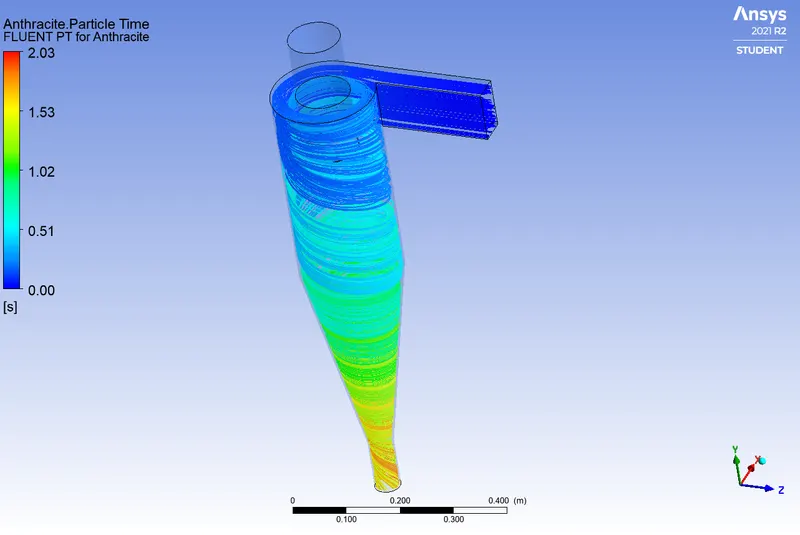
| 1) | Residuals Graph | 2) | Particle residence time | |
|
 |
|||
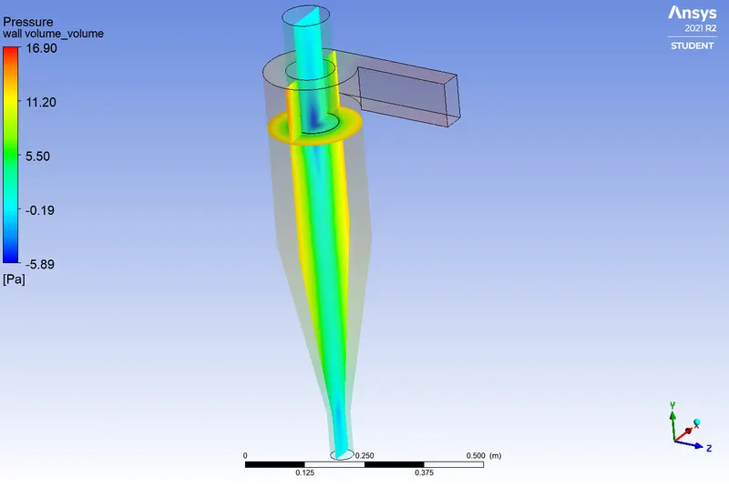
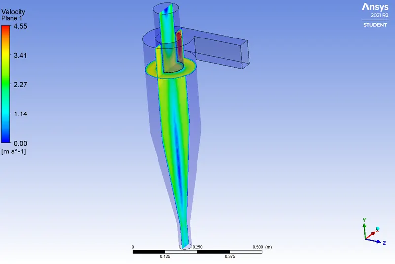
| 3) | Pressure contours on sectional planes | 4) | Velocity contours on sectional planes | |
 |
 |
|||
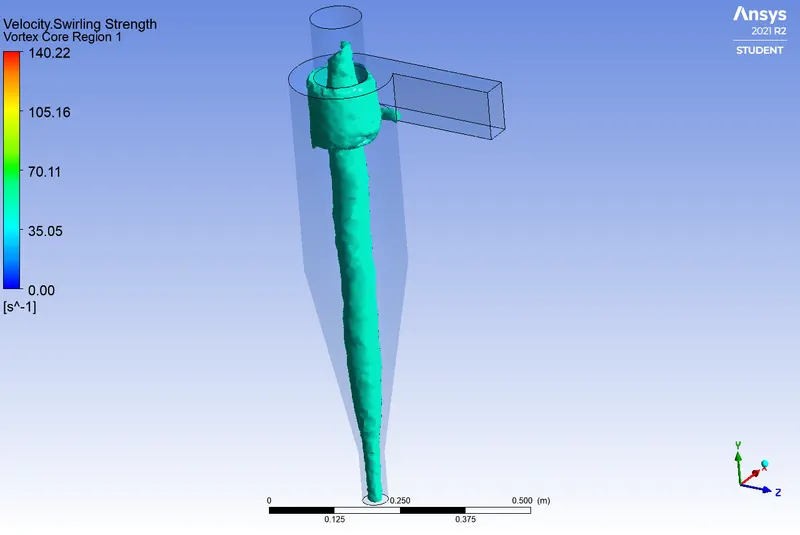
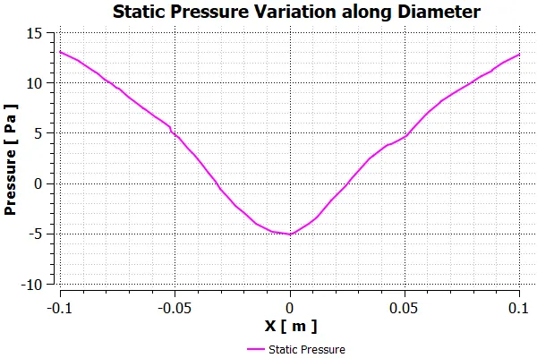
| 5) | Vortex core with strength of level 0.35 ( 49.08 `s^-1`) | 6) | Pressure variation along diameter just below the outlet | |
 |
 |
|||
| 7) | Particle Track Results | 8) | Pressure drop Results | |
| `m_f` = 400 ; `m_e`= 0 ; `m_c`= 400. Thus, Overall Separation Efficiency `eta = frac{400}{400} = 1 = 100%`. |
Max `Delta P` = `16.90 - (-5.89)`= `21.79` Pa; `Delta P` across diameter =`13 - (-5)`= `18` Pa. |
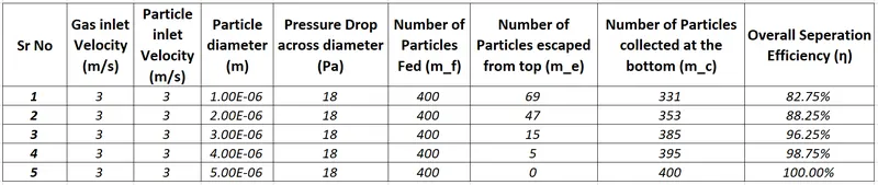
2a) Observation Table:
2b)Graphs:
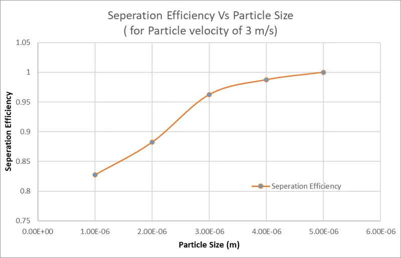
| 1) | Efficiency Vs Particle Size (@ 3 m/s) | 2) | Pressure drop Vs Particle Size (@ 3 m/s) |
 |
 |
||
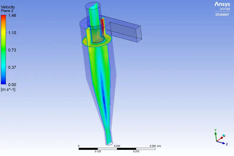
3)Analysis of Cyclone Separator performance with varying particle and gas velocity from 1 `m/s` to 5 `m/s` for 5 `mu m` particle diameter (Same Particle and Gas Velocity).
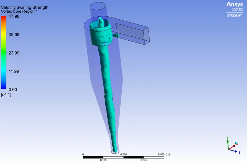
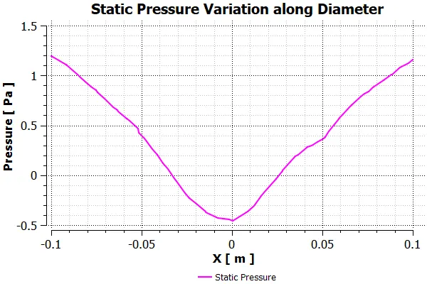
i) Case VI: 5 `mu m` Particle diameter with 1 `m/s` particle and gas velocity.
| 1) | Residuals Graph | 2) | Particle residence time | |
 |
 |
|||
| 3) | Pressure contours on sectional planes | 4) | Velocity contours on sectional planes | |
 |
 |
|||
| 5) | Vortex core with strength of level 0.35 (16.8 `s^-1`) | 6) | Pressure variation along diameter just below the outlet | |
 |
 |
|||
| 7) | Particle Track Results | 8) | Pressure drop results | |
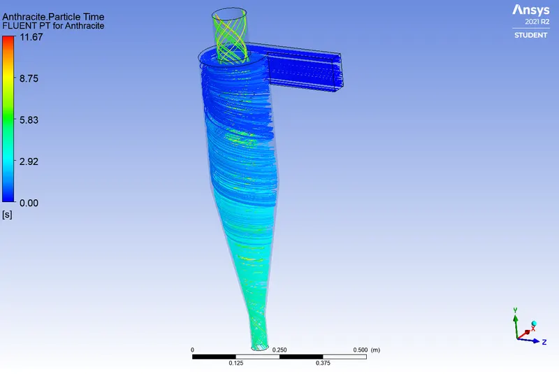
| `m_f` = 400 ; `m_e`= 53 ; `m_c`= 347. Thus, Overall Separation Efficiency `eta = frac{347}{400} = 0.8675 = 86.75%`. |
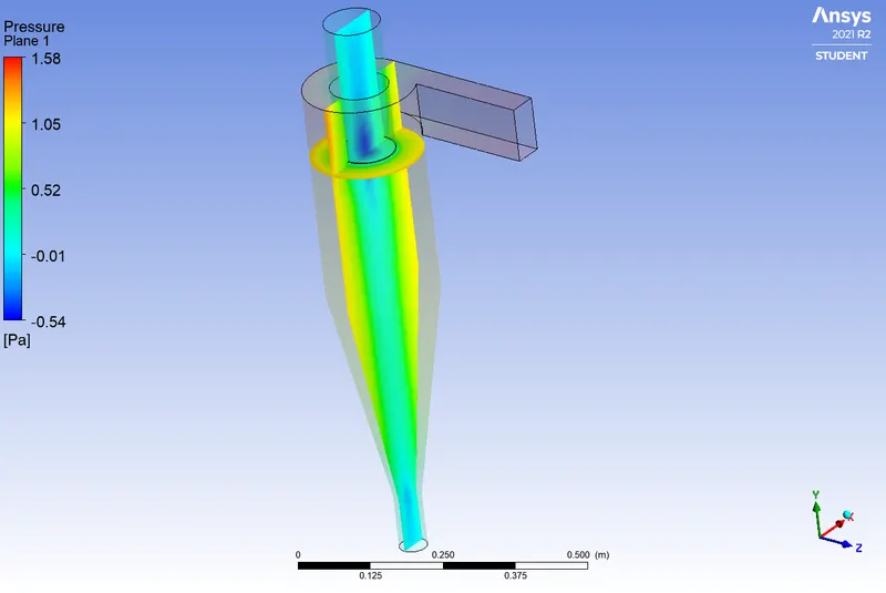
Max `Delta P` = `1.58 - (-0.54)`= `2.12` Pa; `Delta P` across diameter =`1.2 - (-0.45)`= `1.65` Pa. |
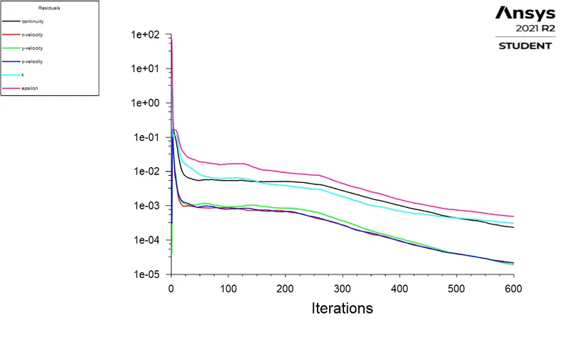
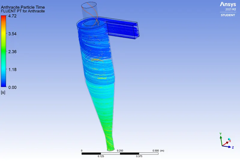
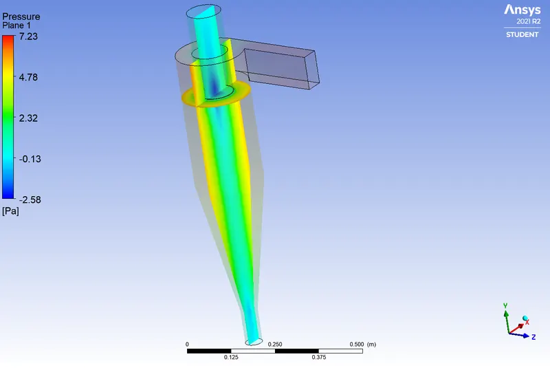
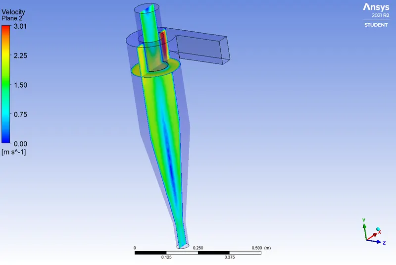
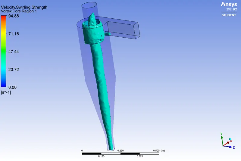
ii) Case VII: 5 `mu m` Particle diameter with 2 `m/s` particle and gas velocity.
| 1) | Residuals Graph | 2) | Particle residence time | |
 |
 |
|||
| 3) | Pressure contours on sectional planes | 4) | Velocity contours on sectional planes | |
 |
 |
|||
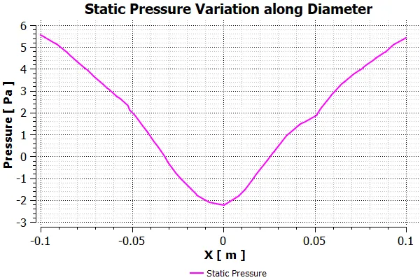
| 5) | Vortex core with strength of level 0.35 (33.21 `s^-1`) | 6) | Pressure variation along diameter just below the outlet | |
 |
 |
|||
| 7) | Particle Track Results | 8) | Pressure drop results | |
| `m_f` = 400 ; `m_e`= 5 ; `m_c`= 395. Thus, Overall Separation Efficiency `eta = frac{395}{400} = 0.9875= 98.75%`. |
Max `Delta P` = `7.23 - (-2.58)`= `9.81` Pa; `Delta P` across diameter =`5.6 - (-2.2)`= `7.8` Pa. |
iii) Case VIII: 5 `mu m` Particle diameter with 3 `m/s` particle and gas velocity.
| 1) | Residuals Graph | 2) | Particle residence time | |
|
|
|||
| 3) | Pressure contours on sectional planes | 4) | Velocity contours on sectional planes | |
|
|
|||
| 5) | Vortex core with strength of level 0.35 ( 49.08 `s^-1`) | 6) | Pressure variation along diameter just below the outlet | |
| |
|
|||
| 7) | Particle Track Results | 8) | Pressure drop Results | |
| `m_f` = 400 ; `m_e`= 0 ; `m_c`= 400. Thus, Overall Separation Efficiency `eta = frac{400}{400} = 1 = 100%`. |
Max `Delta P` = `16.90 - (-5.89)`= `21.79` Pa; `Delta P` across diameter =`13 - (-5)`= `18` Pa. |
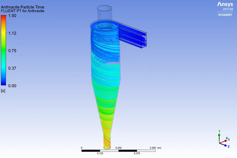
iv) Case IX: 5 `mu m` Particle diameter with 4 `m/s` particle and gas velocity.
| 1) | Residuals Graph | 2) | Particle residence time | |
 |
 |
|||
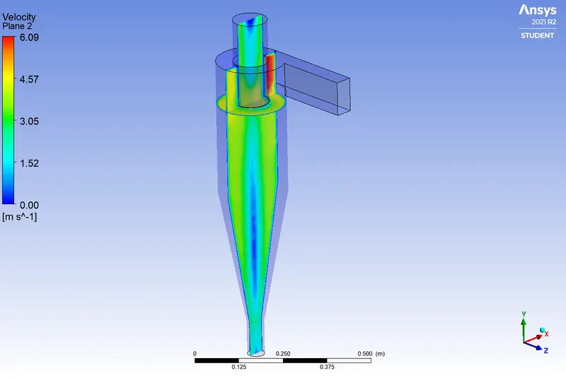
| 3) | Pressure contours on sectional planes | 4) | Velocity contours on sectional planes | |
 |
 |
|||
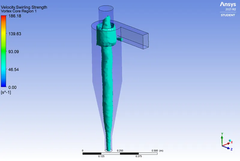
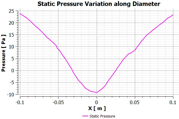
| 5) | Vortex core with strength of level 0.35 (65.16 `s^-1`) | 6) | Pressure variation along diameter just below the outlet | |
 |
 |
|||
| 7) | Particle Track Results | 8) | Pressure drop Results | |
|
`m_f` = 400 ; |
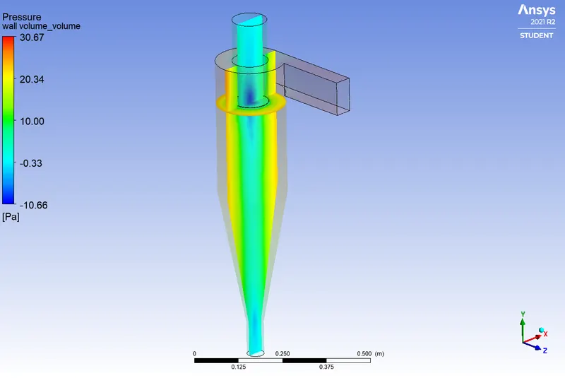
Max `Delta P` = `30.67 - (-10.66)`= `41.33` Pa; `Delta P` across diameter =`24 - (-9)`= `33` Pa. |
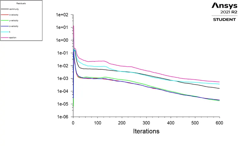
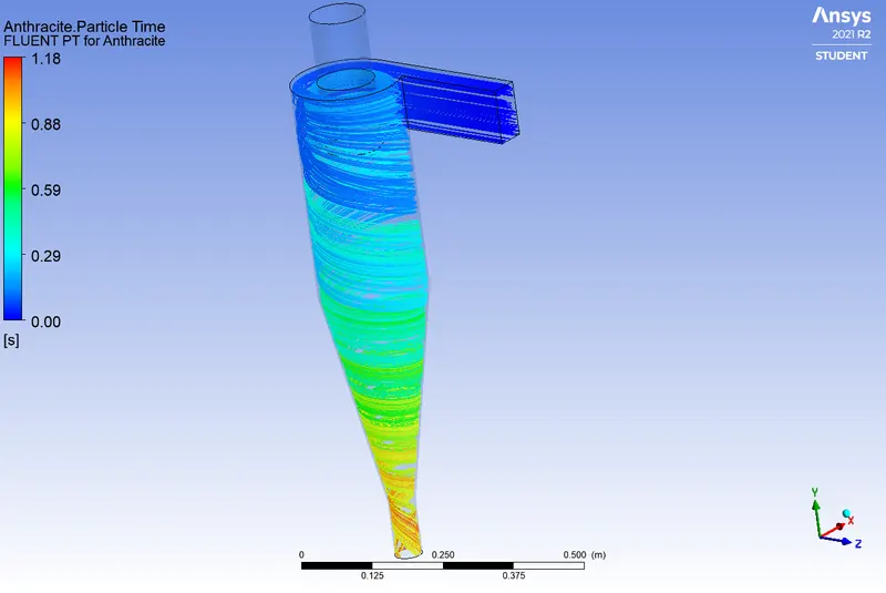
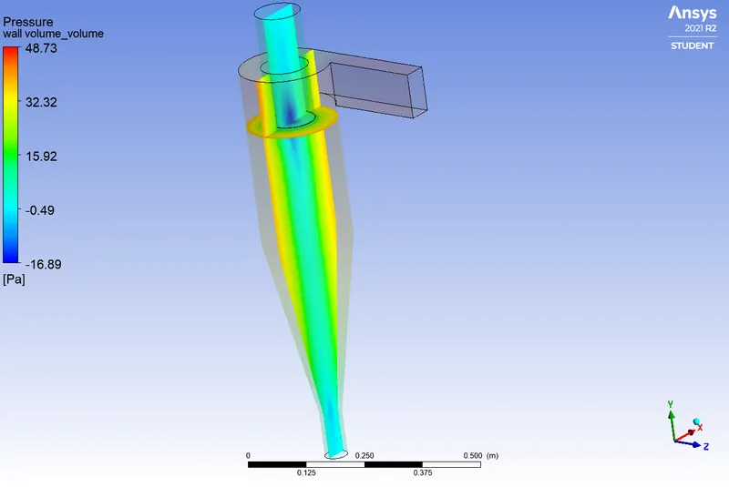
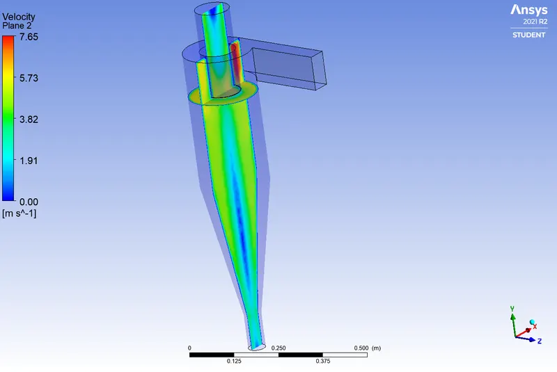
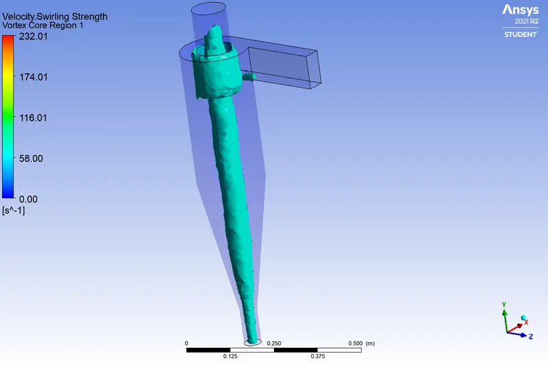
v) Case X: 5 `mu m` Particle diameter with 5 `m/s` particle and gas velocity.
| 1) | Residuals Graph | 2) | Particle residence time | |
 |
 |
|||
| 3) | Pressure contours on sectional planes | 4) | Velocity contours on sectional planes | |
 |
 |
|||
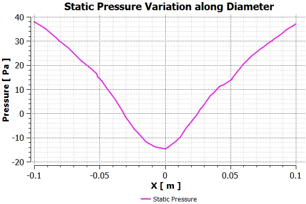
| 5) | Vortex core with strength of level 0.35 (81.2 `s^-1`) | 6) | Pressure variation along diameter just below the outlet | |
 |
 |
|||
| 7) | Particle Track Results | 8) | Pressure drop Results | |
| `m_f` = 400 ; `m_e`= 0 ; `m_c`= 400. Thus, Overall Separation Efficiency `eta = frac{400}{400} = 1 = 100%`. |
Max `Delta P` = `48.73 - (-16.89)`= `65.62` Pa; `Delta P` across diameter =`38 - (-14)`= `52` Pa. |
3a)Observation Table: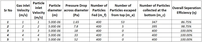
3b)Graphs:
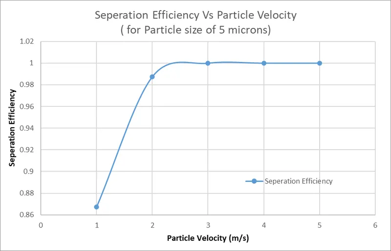
| 1) | Efficiency Vs Particle Velocity (for 5 `mu m` Particle Size) |
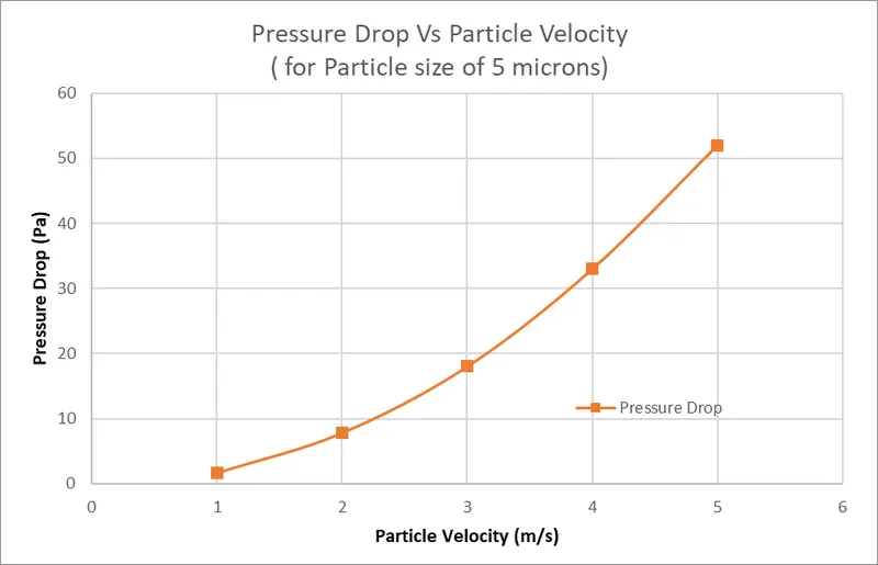
2) | Pressure drop Vs Particle Velocity (for 5 `mu m` Particle Size) |
 |
 |
||
Conclusions:
- From the above results and observations it is clear that for the same inlet velocity pressure drop inside the cyclone separator remains unchanged. If inlet velocity varies linearly the pressure drop inside the cyclone separator varies quadratically, as the pressure is directly proportional to square of the velocity. This can be observed from the graphs for pressure drop.
- From the above results and observations it is clear that the Separation efficiency increases as the particle size increases. This can be observed from the separation efficiency vs particle size graph for particle velocity of 3 m/s.
- Also the separation efficiency of the cyclone separator increases as the inlet velocity increases, this can be observed from the graph of separation efficiency vs particle velocity for the particle size of 5 microns.
References:
[1] John Dirgo & David Leith (1985) Cyclone Collection Efficiency: Comparison of Experimental Results with Theoretical Predictions, Aerosol Science and Technology, 4:4, 401-415, DOI: 10.1080/02786828508959066 .
[2]Jolius Gimbun et al.(2005) A CFD Study on the Prediction of Cyclone Collection Efficiency, International Journal for Computational Methods in Engineering Science and Mechanics, 161-168, DOI:10.1080/15502280590923649 .
[3]B. Wang et al.(2006) Numerical study of gas–solid flow in a cyclone separator, Applied Mathematical Modelling 30, 1326–1342,doi:10.1016/j.apm.2006.03.011 .