Week 8- Moving zones approach in Fluent
Aim:
(i)To study about aprroaches involved in model moving zones.
(ii)To study about approach used to model unsteady phenomena.
(iii)To study about velocit profile by simulating the rotary motion of geometry given.
Introduction:
Fluent:
In the early 1980s, from the buildings of Sheffield University with contributions from multiple personalities, Ansys Fluent became the first commercial computational fluid dynamics (CFD) software to have a graphical user interface and workflow rather than a command-line input. The popularity of Fluent increased year after year, along with its adoption in the industry.In May 2006, Fluent Inc. was acquired by Ansys. Since joining the Ansys family, we have relentlessly pushed the envelope of performance, accuracy, and productivity of Fluent, bringing cutting-edge innovations that have helped engineers overcome the most challenging design obstacles imaginable when dealing with fluid dynamics problems.2014: GPU-Accelerated Offloading and Adjoint Solver.While graphics processing unit (GPU) technologies are in the spotlight today, the concept of using GPUs as CFD accelerators was introduced in Fluent in 2014 with the NVIDIA AmgX solver. Bear with us in this time-travel scenario, because in 2022, Fluent will be the first commercial CFD software to introduce an unstructured finite volume, fully resident multi-GPU solver, overcoming the offloading limitations and disrupting the market for CFD simulations.The Adjoint solver was firs introduced in Fluent in 2014 to revolutionize insights from CFD simulations by using the adjoint sensitivities to drive intelligent design changes that are not intuitive to a designer. Since its inception, the reliability and usability of the Adjoint solver has consistently evolved into a comprehensive product optimization framework.Optimize designs through automated shape optimization using the Adjoint solver, introduced in 2014.2016: Fluent Breaks a Supercomputing Record of 170,000 Cores.In 2016, Cray Inc. and the High Performance Computing Center (HLRS) of the University of Stuttgart set a new supercomputing world record by scaling Fluent to more than 172,000 computer cores, enabling organizations to create innovative and groundbreaking complete virtual prototypes of their products faster and more efficiently than ever.Another cutting-edge innovation for a commercial CFD software was the introduction of patented polyhedral unstructured mesh adaptation (PUMA) in 2017. This adaption technique automatically and dynamically refines the mesh to track fine details in the flow. As a result, engineers can get the accuracy they need, where they need it, to capture simulation details while leaving courser mesh elsewhere for faster solve times.Accelerate solve times by automatically refining a mesh to resolve fine details while leaving coarser mesh in place using polyhedral unstructured mesh adaptation (PUMA), introduced in 2017.The same year, the stress-blended eddy simulation (SBES) turbulence model overcame inherent problems with hybrid RANS-LES simulations. Large-eddy simulation (LES) is impractically expensive in the near-wall region while Reynolds-averaged Navier-Stokes (RANS) models are well-suited for wall boundary layers. Hybrid RANS-LES models provide efficient near-wall modeling using a RANS turbulence model and a high-fidelity solution away from walls using an LES approach, but switching between the two traditionally suffered from mesh dependency and false mesh-induced flow separation. The SBES model developed by Ansys introduced a unique and proprietary shielding function to overcome these problems, resulting in a reliable and efficient scale-resolving turbulence model that engineers can trust.Transitioning among varying types of mesh elements in complex geometries while retaining mesh quality has long been a major meshing challenge, particularly when transitioning from boundary layer prisms to hex elements away from walls. In 2018, Fluent introduced Mosaic meshing to address this challenge by automatically connecting different types of meshes with high-quality polyhedral elements. The resulting simulations were dramatically faster with greater solution accuracy while using less RAM.Ferrari Competizioni GT increases simulation productivity by 300% using Mosaic meshing technology, introduced in 2018.The same year, the spray breakup model was the first commercial implementation of volume of fluid (VOF) to discrete particle method (DPM) transition for multiphase simulations, such as spray breakup. In this model, distinct droplets in the VOF simulation are detected and replaced by DPM (i.e., mass-point) particles, and the mesh is coarsened accordingly.Efficiently simulate spray breakup using the volume of fluid (VOF) to discrete particle method (DPM) hybrid multiphase model, introduced in 2017.In 2019, the Ansys turbulence team introduced a generalized k-ω turbulence (GEKO) model with tunable coefficients. GEKO’s tunable coefficients can be adjusted over a wide range to match specific physical effects while maintaining the underlying model calibration. No other turbulence model has enough flexibility to match experimental data over a large set of test cases — even if tuned by a turbulence model expert — while GEKO’s coefficients provide that flexibility. The GEKO model can even be tuned to scale-resolving simulation results, such as those using the SBES turbulence model. The GEKO turbulence model is exclusively available in Ansys fluids applications.In 2020, Fluent was the first commercial software to showcase an Eulerian multiphase transition method based on the algebraic interfacial area density (AIAD) approach. This method is suitable for a range of applications such as loss of coolant scenarios in pressurized-water reactors, with strong agreement with experimental data compared to alternative methods.Gas‒liquid flow with droplet entrainment and re-absorption using AIAD transition, introduced in 2020.The same year, Fluent introduced the transient simulation of lithium (Li)-ion transport during battery charging/discharging providing a complete commercial solution for 3D electrochemistry of Li-ion batteries.As previously mentioned, the VOF to DPM transition was first introduced in Fluent in 2018 with the spray breakup model. In 2021, Fluent made this transition bidirectional, supporting the inverse DPM-to-VOF transition and completing it with the transition to Eulerian wall film (EWF). In the bidirectional VOF-to-DPM-to-EWF model, DPM particles falling onto a free liquid surface transition back into VOF formulation and the mass-point particles are replaced by mesh-resolved VOF liquid.Efficiently simulate breakup, pooling, and thinning of multiphase flows using the bidirectional VOF-to-DPM-to-EWF feature, introduced in 2021.The same year, Fluent introduced AI/ML artificial intelligence (AI)/machine learning (ML) turbulence tuning, in which the GEKO coefficients are tuned with ML algorithms rather than manually. This enables engineers to use a scale-resolving turbulence model such as SBES to generate a high-fidelity solution. They then can use ML to tune the GEKO coefficients throughout the 3D flow field so that subsequent design iterations can use the much-faster GEKO model while retaining accuracy that approaches the scale-resolving solution.As previously mentioned, Fluent has been a trailblazer in the use of GPU technology for simulation, and in 2022 it took it to a new level with the introduction of a native multi-GPU solver. This brand-new multi-GPU solver provides many benefits for steady-state and transient CFD simulations, including reducing simulation solve time, hardware costs, and power consumption with the same accuracy of the CPU solvers and without all the limitation of GPU offloading we previously mentioned.Six high-end GPUs provide the same performance as more than 2,000 CPUs when using the native multi-GPU solver, introduced in 2022.Finally, Fluent introduced PyFluent, an open-source library to access all Fluent commands from pre- to post-processing using Python. PyFluent is designed to combine a robust community of peers, a programming language such as Python that encourages reuse, and Ansys' state-of-the-art simulation stack to create endless possibilities.
Moving Zones:
These are some of the Applications such as rotary pumps,valves e.t.c..,needs a Computational Fluid Dynamics to estimate a paramaters and to visualise the flow patterns.
Rotary Pumps:
Rotary pumps are positive displacement pumps that use rotating components to trap and transport fluid. They are widely used in various industries due to their high efficiency, reliability, and ability to handle high viscosity fluids. we will discuss the types of rotary pumps and their working principle
1.Gear Pump
2.screw pump
3.Vane pump
4.Lobe pump
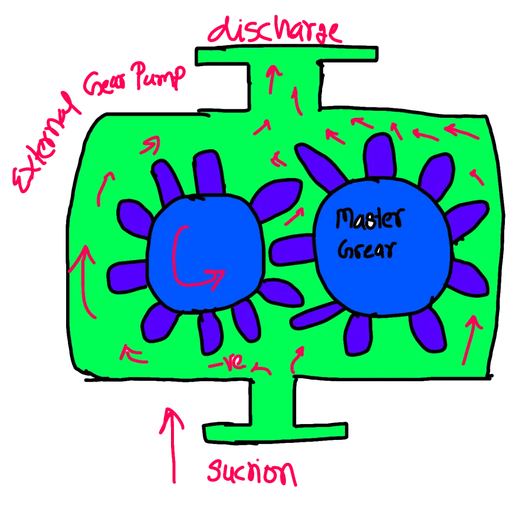
Gear Pump:The gear pump works by trapping the fluid between the teeth of the two gears and the casing. As the gears rotate, the fluid is transported from the suction port to the discharge port. The flow rate of the pump is proportional to the size of the gears and the speed of rotation.
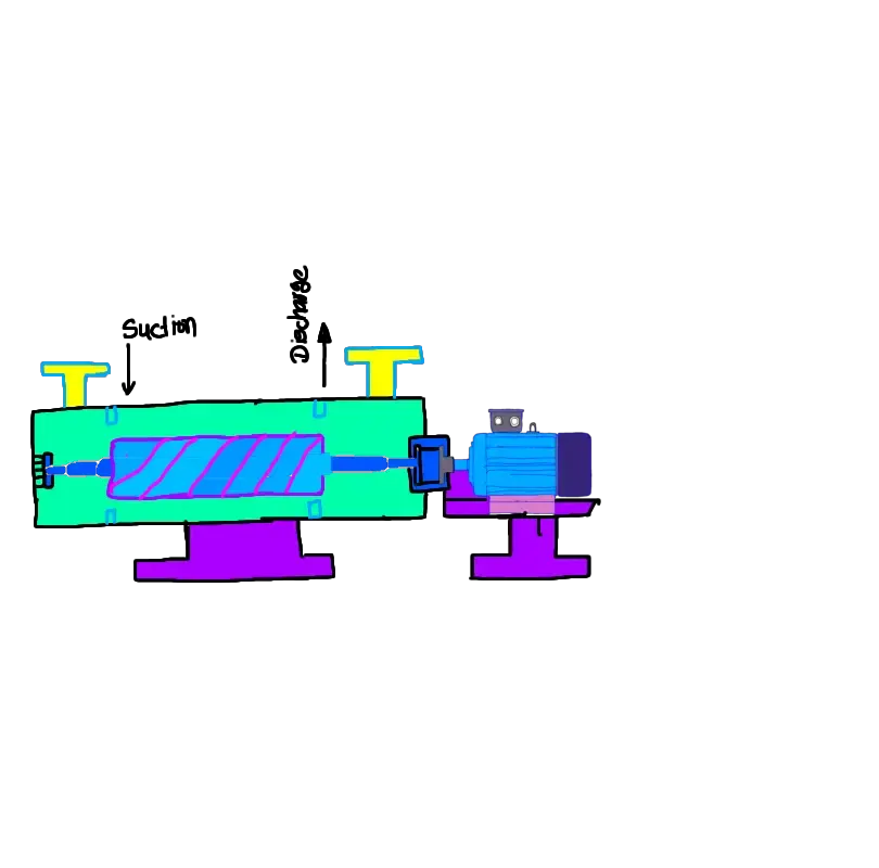
Screw Pump:Screw pumps work by trapping the fluid between the screws and transporting it along the length of the screws. The screws can be helical or meshing, and the pump can have a single or double screw design. The flow rate of the pump is proportional to the size of the screws and the speed of rotation.
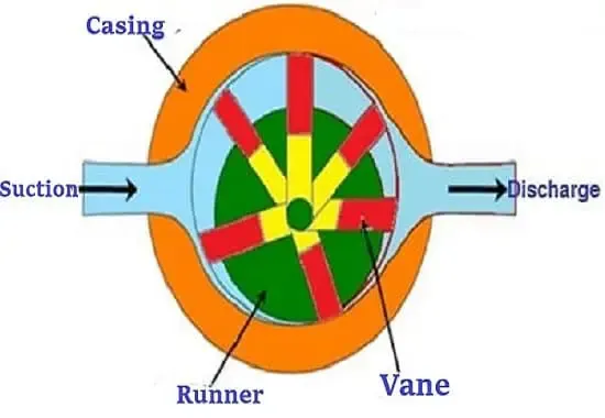
Vane Pump:Vane pumps work by creating a vacuum that draws the fluid into the pump. The rotor with sliding vanes traps the fluid between the rotor and the casing. As the rotor rotates, the vanes slide in and out, creating a vacuum that draws the fluid into the pump. The flow rate of the pump is proportional to the size of the vanes and the speed of rotation.
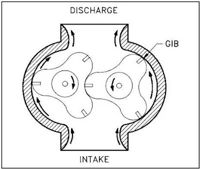
Lobe Pump:Lobe pumps work by trapping the fluid between the lobes and the casing. As the lobes rotate, the fluid is transported from the suction port to the discharge port. The flow rate of the pump is proportional to the size of the lobes and the speed of rotation.
on all these ,we can observe the common thing is the rotating component due to this fluid zones will changing (or) moving near the rotor components.
Several applications needs the Moving zones.In this,going to discuss abount the moving zones
Theory:
modelling of different Approaches of Moving Zones:
The Moving zone will be approached in two ways.
(i)Moving Reference Frame
(ii)Mesh Motion
Moving Reference Frame:Ansys Fluent solves the equations of fluid flow and heat transfer, by default, in a stationary (or inertial) reference frame. However, there are many problems where it is advantageous to solve the equations in a moving (or non-inertial) reference frame. Such problems typically involve moving parts (such as rotating blades, impellers, and similar types of moving surfaces), and it is the flow around these moving parts that is of interest. In most cases, the moving parts render the problem unsteady when viewed from the stationary frame. With a moving reference frame, however, the flow around the moving part can (with certain restrictions) be modeled as a steady-state problem with respect to the moving frame.Ansys Fluent’s moving reference frame modeling capability allows you to model problems involving moving parts by allowing you to enable moving reference frames in selected cell zones. When a moving reference frame is activated, the equations of motion are modified to incorporate the additional acceleration terms that occur due to the transformation from the stationary to the moving reference frame.By solving these equations in a steady-state manner, the flow around the moving parts can be modeled.
The principal reason for employing a moving reference frame is to render a problem that is unsteady in the stationary (inertial) frame, steady with respect to the moving frame. For a steadily moving frame (for example, the frame speed is constant), it is possible to transform the equations of fluid motion to the moving frame such that steady-state solutions are possible. By default, Ansys Fluent permits the activation of a moving reference frame with a steady speed. If the speed is not constant, the transformed equations will contain additional terms . It should also be noted that you can run an unsteady simulation in a moving reference frame with constant speed. This would be necessary if you wanted to simulate, for example, vortex shedding from a rotating fan blade. The unsteadiness in this case is due to a natural fluid instability (vortex generation) rather than induced from interaction with a stationary component.
For many problems, it may be possible to refer the entire computational domain to a single moving reference frame. This is known as the single reference frame (or SRF) approach. The use of the SRF approach is possible; provided the geometry meets certain requirements. For more complex geometries,it may not be possible to use a single reference frame. In such cases, you must break up the problem into multiple cell zones, with well-defined interfaces between the zones. This is the multiple reference frame (or MRF) approach and is discussed in The Multiple Reference Frame Model. If unsteady interaction between the stationary and moving parts is important, you can employ the sliding mesh approach to capture the transient behavior of the flow. The sliding meshing model will be discussed
SRF (Single Reference Frame) Modelling:
Many problems permit the entire computational domain to be referred to a single moving reference frame. In such cases, the equations given in Equations for a Moving Reference Frame are solved in all fluid cell zones. Steady-state solutions are possible in SRF models provided suitable boundary conditions are prescribed. In particular, wall boundaries must adhere to the following requirements:
• Any walls that are moving with the reference frame can assume any shape. An example would be the blade surfaces associated with a pump impeller. The no slip condition is defined in the relative frame such that the relative velocity is zero on the moving walls.
• For a rotating problem, you can define walls that are non-moving with respect to the stationary coordinate system, but these walls must be surfaces of revolution about the axis of rotation. Here the no slip condition is defined such that the absolute velocity is zero on the walls. An example of this type of boundary would be a cylindrical wind tunnel wall that surrounds a rotating propeller.
Rotationally periodic boundaries may also be used, but the surface must be periodic about the axis of rotation. As an example, it is very common to model flow through a blade row of a turbomachine by assuming the flow to be rotationally periodic and using a periodic domain about a single blade. This permits good resolution of the flow around the blade without the expense of modeling all blades in the blade row .
Flow boundary conditions in Ansys Fluent (inlets and outlets) can, in most cases, be prescribed in either the stationary or moving frames. For example, for a velocity inlet, one can specify either the relative velocity or absolute velocity, depending on which is more convenient.
Flow in Multiple Moving References:Many problems involve multiple moving parts or contain stationary surfaces which are not surfaces of revolution. For these problems, you must break up the model into multiple fluid/solid cell zones, with interface boundaries separating the zones. Zones that contain the moving components can then be solved using the moving reference frame equations ,whereas stationary zones can be solved with the stationary frame equations.
MRF Model:
The MRF model , the simplest of the two approaches for multiple zones. It is a steady-state approximation in which individual cell zones can be assigned different rotational and/or translational speeds. The flow in each moving cell zone is solved using the moving reference frame equations. If the zone is stationary , the equations reduce to their stationary forms. At the interfaces between cell zones, a local reference frame transformation is performed to enable flow variables in one zone to be used to calculate fluxes at the boundary of the adjacent zone.It should be noted that the MRF approach does not account for the relative motion of a moving zone with respect to adjacent zones (which may be moving or stationary); the mesh remains fixed for the computation. This is analogous to freezing the motion of the moving part in a specific position and observing the instantaneous flowfield with the rotor in that position. Hence, the MRF is often referred to as the “frozen rotor approach.” While the MRF approach isclearly an approximation, it can provide a reasonable model of the flow for many applications. For example, the MRF model can be used for turbomachinery applications in which rotor-stator interaction is relatively weak, and the flow is relatively uncomplicated at the interface between the moving and stationary zones. In mixing tanks, for example, since the impellerbaffle interactions are relatively weak, large-scale transient effects are not present and the MRF model can be used. Another potential use of the MRF model is to compute a flow field that can be used as an initial condition for a transient sliding mesh calculation. This eliminates the need for a startup calculation.The multiple reference frame model should not be used, however, if it is necessary to actually simulate the transients that may occur in strong rotor-stator interactions, the sliding mesh model alone should be used.
The following limitations exist when using the MRF approach:
• The interfaces separating a moving region from adjacent regions must be oriented such that the component of the frame velocity normal to the boundary is zero. This means that for a translationally moving frame, the moving zone’s boundaries must be parallel to the translational velocity vector. For rotating problems, the interfaces must be surfaces of revolution about the axis of rotation defined for the fluid zone. Impeller , this requires the dashed boundary to be circular
• The use of multiple reference frames is meaningful only for steady flow. However,Ansys Fluent will allow you to solve an unsteady flow when multiple reference frames are being used. In this case, unsteady terms are added to all the governing transport equations. You should carefully consider whether this will yield meaningful results for your application, because, for unsteady flows, a sliding mesh calculation will generally yield more meaningful results than an MRF calculation.
• By default, pathlines and particle trajectories drawn by Ansys Fluent use the velocity relative to the reference frame motion of the cell zone. However, for particle trajectories, you can change the reference frame by either selecting Track in Absolute Frame in the Numerics tab of the Discrete Phase Model dialog box or using the text command define/models/dpm/options/track-in-absolute-frame.
• You cannot accurately model axisymmetric swirl in the presence of multiple reference frames using the relative velocity formulation. This is because the current implementation does not apply the transformation used in Equation , to the swirl velocity derivatives.For this situation, the absolute velocity formulation should be used.
• Translational and rotational velocities are assumed to be constant (time varying , are notallowed).
• The relative velocity formulation cannot be used in combination with the MRF and mixture models. For such cases, use the absolute velocity formulation
• You must not have a single interface between reference frames where part of the interface is made up of a coupledtwo-sided wall, while another part is not coupled. In such cases, you must break the interface up into two interfaces: one that is a coupled interface, and the other that is a standard fluid-fluid interface. A NonConformal Mesh in Ansys Fluent for the steps involved in setting up a coupled interface
Mixing Plane Model:
In the mixing plane approach, each fluid zone is treated as a steady-state problem. Flow-field data from adjacent zones are passed as boundary conditions that are spatially averaged or “mixed” at the mixing plane interface. This mixing removes any unsteadiness that would arise due to circumferential variations in the passage-to-passage flow field (for example, wakes, shock waves, separated flow), therefore yielding a steady-state result. Despite the simplifications inherent in the mixing plane model, the resulting solutions can provide reasonable approximations of the time-averaged flow field.
The essential idea behind the mixing plane concept is that each fluid zone is solved as a steadystate problem. At some prescribed iteration interval, the flow data at the mixing plane interface are averaged in the circumferential direction on both the stator outlet and the rotor inlet boundaries.The Ansys Fluent implementation gives you the choice of three types of averaging methods: areaweighted averaging, mass averaging, and mixed-out averaging. By performing circumferential averages at specified radial or axial stations,“profiles” of boundary condition flow variables can be defined. These profiles—which will be functions of either the axial or the radial coordinate, depending on the orientation of the mixing plane—are then used to update boundary conditions along the two zones of the mixing plane interface. profiles of averaged are total pressure , direction cosines of the local flow angles in the radial, tangential, and axial directions , total temperature , turbulence kinetic energy, and turbulence dissipation rate are computed at the rotor exit and used to update boundary conditions at the stator inlet.Likewise, a profile of static pressure , direction cosines of the local flow angles in the radial,tangential, and axial directions , are computed at the stator inlet and used as a boundary condition on the rotor exit.Passing profiles in the manner described above assumes specific boundary condition types haveeen defined at the mixing plane interface. The coupling of an upstream outlet boundary zone with a downstream inlet boundary zone is called a “mixing plane pair”
Sliding Mesh Model:
This model is a combination of moving mesh and multiple reference frames.The sliding mesh model is a special case of general dynamic mesh motion wherein the nodes move rigidly in a given dynamic mesh zone. Additionally, multiple cells zones are connected with each other through non-conformal interfaces. As the mesh motion is updated in time,the non-conformal interfaces are likewise updated to reflect the new positions each zone. It is important to note that the mesh motion must be prescribed such that zones linked through non-conformal interfaces remain in contact with each other (that is,“slide” along the interface boundary) if you want fluid to be able to flow from one mesh to the other. Any portion of the interface where there is no contact is treated as a wall
Approach use to model Unsteady Phenomena:
The MRF model is applicable when the flow at the interface between adjacent moving/stationary zones is nearly uniform (“mixed out”).If the flow at this interface is not uniform, the MRF model may not provide a physically meaningful solution. The sliding mesh model may be appropriate for such cases, but in many situations it is not practical to employ a sliding mesh. For example, in a multistage turbomachine, if the number of blades is different for each blade row, a large number of blade passages is required in order to maintain circumferential periodicity. Moreover, sliding mesh calculations are necessarily unsteady, and therefore require significantly more computation to achieve a final, time-periodic solution. For situations where using the sliding mesh model is not feasible, the mixing plane model can be a cost-effective alternative.So it is clear unsteady phenomena solved by Sliding mesh (or) special type dynamic mesh motion
Simulation:
i.Geometry has a domain contains a lot of airfoil shape at angles.
ii.in this simulation domain contains airfoil shapes should rotate at 250 rpm about its axis.
Two ways to solve
1.Rotating reference frame-used to solve for steady state.
2.Rotating mesh about its axis-used to solve the unsteady state and compute slowly.
Rotating Reference frame is selected
iii. Laminar or turbulent flow will be determined with the help of rotational reynolds number
Based on this,flow is turbulent.
determing wether flow is compressible or incompressible based on the mach number
mach number <0.3 then flow is incompressible.
iv.Model will be determined
`K-omega` standard-free shear flows, including far wakes, mixing layers, strongly separated flows, as well as plane, round, and radial jets,Higher Ma flows,high degree of swirl,both near wall and steam turbulence
`K-omega`SST- adverse pressure gradient,Separated flows,Turbulent Heat transfer ,Reynolds number(High and low) and aerospace applications
`K-epsilon`Standard-, Free shear layer flow, Flows with nonexistent to small pressure gradients , Simplified case of boundary layer flow over a flat plate, Channel flow for Re in the range of 6000 to 150,000 ,free jet
`K-epsilon` RNG-rapidly strained flows,the effect of swirl on turbulence , enhancing accuracy for swirling flows.
`K-epsilon`Realizable- strong streamline curvature, vortices, and rotation
For rotation flows,`K-epsilon` Realizable model will be better suited.
v.Wall functions has to select
standard wall functions-boundary layer lies entirely within loglaw region.
Scalable wall functions -avoid the deterioration of standard wall functions under grid refinement below `y^+<11`
In addition to the standard wall function described above (which is the default near-wall treatment) a two-layer-based, non-equilibrium wall function
Enhanced Wall Treatment for the -equation is a near-wall modeling method that combines a twolayer model with so-called enhanced wall functions. If the near-wall mesh is fine enough to be able to resolve the viscous sublayer (typically with the first near-wall node placed at ), then the enhanced wall treatment will be identical to the traditional two-layer zonal model.
menter lechner wall functions-The goal of a -insensitive near-wall treatment is the -independent prediction of the wall shear stress and wall heat flux (assuming a sufficient resolution of the boundary layer). The formulation should switch gradually from wall functions to a low-Re formulation when the mesh is refined. This also requires a blending of various quantities between the viscous sublayer and the logarithmic region.
Enhanced wall treatment will be selected to resolve the boundaries in viscous sub layer.
Vi.Pressure-velocity coupling Scheme
simple-If a steady-state problem is being solved iteratively, it is not necessary to fully resolve the linear pressure-velocity coupling, as the changes between consecutive solutions are no longer small
SIMPLEC algorithm is seen to converge 1.2-1.3 times faster than the SIMPLE algorithm
PISO is a pressure-velocity calculation procedure for the Navier-Stokes equations developed originally for non-iterative computation of unsteady compressible flow, but it has been adapted successfully to steady-state problems.
Coupled-Using the coupled approach offers some advantages over the non-coupled or segregated approach. The coupled scheme obtains a robust and efficient single phase implementation for steady-state flows, with superior performance compared to the segregated solution schemes.
Coupled scheme is selected due to superior performance for steady flows.
Vii.Spatial discretisation schemes
First order upwind scheme-When first-order accuracy is desired, quantities at cell faces are determined by assuming that the cell-center values of any field variable represent a cell-average value and hold throughout the entire cell
Second order upwind scheme-when second order accuracy is desired, quantities at cell faces are computed using a multidimensional linear reconstruction approach
QUICK scheme-For quadrilateral and hexahedral meshes, where unique upstream and downstream faces and cells can be identified, Ansys Fluent also provides the QUICK scheme for computing a higher-order value of the convected variable at a face
MUSCL Scheme-This third-order convection scheme was conceived from the original MUSCL (Monotone Upstream Centered Schemes for Conservation Laws) by blending a central differencing scheme and second-order upwind scheme.
Second order upwind scheme is selected because of higher order for tetra mesh.
viii.Gradients and derivatives scheme:
Green-Gauss Cell-Based-When the Green-Gauss theorem is used to compute the gradient of the scalar at the cell center
Green-Gauss Node-Based-the node-based gradient is known to be more accurate than the cell-based gradient particularly on irregular (skewed and distorted) unstructured meshes, however, it is relatively more expensive to compute than the cell-based gradient scheme
Least Squares Cell-Based-On irregular (skewed and distorted) unstructured meshes, the accuracy of the least-squares gradient method is comparable to that of the node-based gradient . However, it is less expensive to compute the least-squares gradient than the node-based gradient.
Least Squares cell based is used because using a unstructured meshes.
Procedure:
1.Imported the mesh file on the fluent by file->read->mesh option is selected.
2.Domain->mesh->check->perform mesh check option is selected to check the mesh.
3.Domain->mesh->quality->evaluate mesh quality option is selected to see values of two most important mesh parameters,1.Minimum orthogonal quality,2.Maximum Aspect ratio.
4.physics->models->viscous is selected then viscous model dialog box appears K-`epsilon` Realizanle model is selected and Enhanced wall treatment and then click ok.
5.Physics->materials->create/edit is selected then create/edit materials window appears .Fluent fluid materials drop-down list is selected then loaded materials from the fluent database is seen.
6.physics->zones->cellzones is selected,then zone is selected as fluid,then frame motion checkbox turned on,frame rotation speed about origin is 250 RPM and then apply.
7.physics->zones->Boundaries is selected,then airfoil is selected then edited on the wall dialog box,then airfoil set it as moving wall ,relative to the cell adjacent zone ,rotational ,then click apply.
8.solution -> methods is selected,then checked the spatial discretisation schemes all parameter schemes must be second order upwind.
9.solution->controls,then the flow courant number changed to 10.
10.Solution->initialisation,then Hybrid is selected under the method and click on t=0 initialise button.
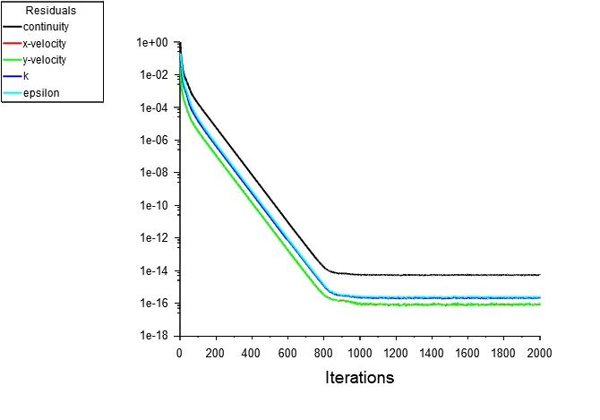
11.solution->reports->residualsis selected then check convergence checkbox is deselected ,then ok
12.solution->run calculation,then no of iterations changed to 2000 and then hit calculate.
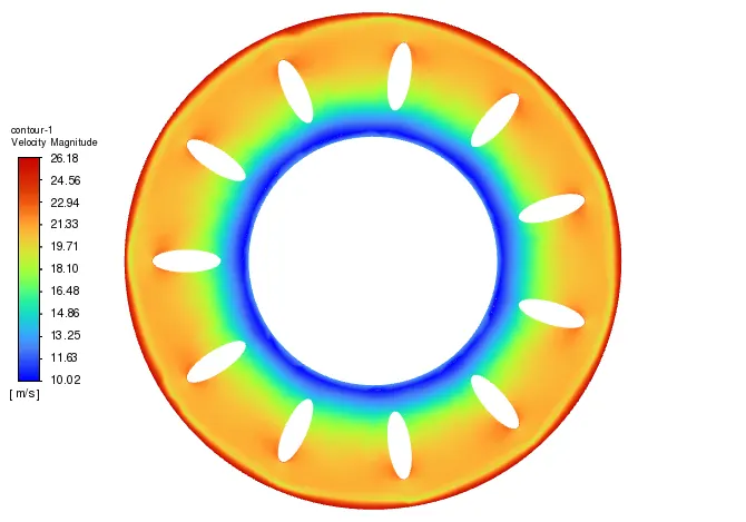
13.Results->graphics->contour->new ,then contour dialog box appears then velocity parameter has been selected.
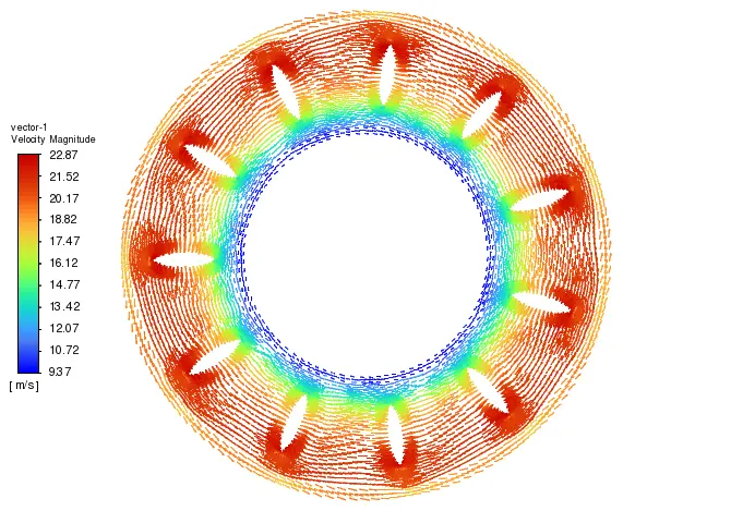
14. Results->graphics->vector->new ,then vector dialog box appears then velocity parameter has been selected.
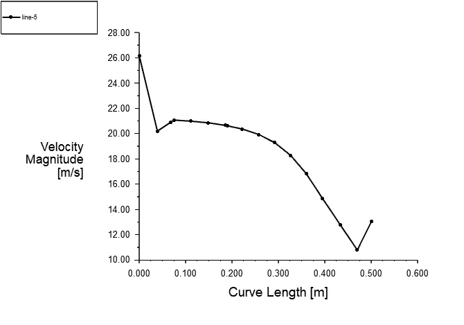
15.Results->surface->create->line/Rake ,then line/rake dialog box appears and then click ok.
16.Results->plots->xy plots->new then solution xyplots window appears then parameters selected and then click ok.
Plots:
Conclusion:
(i)Studied about the approaches of moving Zones and models in Ansys Fluent.
(ii)Learned about the model that used to solve the unsteady moving zones
(iii)Simulated the rotating reference frame approach using ANSYS Fluent.
(iv)Simulation converged after 1000 iterations.
(v)Simulation shows that velocity is high near the outer wall and velocity is low near the inner wall
(vi)Flow across the domain has plotted the velocity,it shows velocity increasing from inner surface