Week 3 - Taylor table method and Matlab code

Aim

i.To derive a three different schemes of fourth order approximation for second order derivative

ii.To compute and compare the three different schemes for a function `e^x*cos x`

Introduction

To analyze a Fluid flow,it is necessary to discretise the object and solving the discretised object with the help of three methods (i)Finite Difference Methods(FDM) (ii)Finite Volume Method(FVM) (iii)Finite Element Method(FEM). In numerical analysis, finite-difference methods (FDM) are a class of numerical techniques for solving differential equations by approximating derivatives by using a Finite Differences.The finite volume method (FVM) is a method for representing and evaluating partial differential equations in the form of algebraic equations.The FEM is a particular numerical method for solving partial differential equations in two or three space variables (i.e., some boundary value problems).

Derivation

Deriving a fourth order approximation for second order derivative by using a three schemes

(i)Central differencing

(ii)Skewed right-sided difference

(iii)skewed left-sided difference

i.central differencing

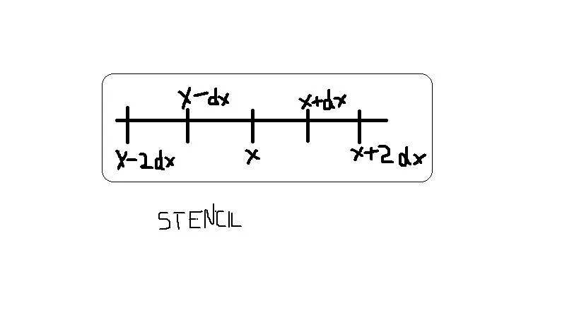
The central differencing scheme is a finite difference method that optimizes the approximation for the differential operator in the central node of the considered patch and provides numerical solutions to differential equations

In Central differencing use a symmetric stencil,stencil is a geometric arrangement of a nodal group that relate to the point of interest by using a numerical approximation routine

it was clear to derive a fourth order approximation for second order derivative with the help of taylor table method

`frac{d^2y}{dx^2}=a*f(x-2dx)+b*f(x-dx)+c*f(x)+d*f(x+dx)+e*f(x+2dx)`

	f(x)	`f'(x)*dx`	`f''(x)*dx^2`	`f'''(x)*dx^3`	`f''''(x)*dx^4`
f(x-2dx)	a	`-2*a`	`frac{4*a}{2}`	`frac{-8*a}{6}`	`frac{16*a}{24}`
f(x-dx)	b	-b	`frac{b}{2}`	`frac{-b}{6}`	`frac{b}{24}`
f(x)	c	0	`0`	0	0
f(x+dx)	d	d	`frac{d}{2}`	`frac{d}{6}`	`frac{d}{24}`
f(x+2dx)	e	`2*e`	`frac{4*e}{2}`	`frac{8*e}{6}`	`frac{16*e}{24}`
	0	0	1	0	0

from the above taylor table gives a 5 set of unkowns,we can calculate by using matrix inversion method

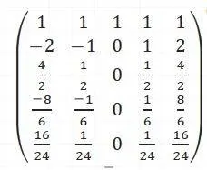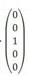A= B= X=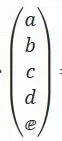

A matrix is transpose of taylor table

B matrix is the balancing of second order derivative

X are the unknowns

X=`A^-1*B`

=

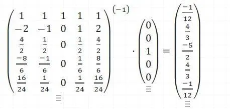
from the result we know that a=e=-0.0833,b=d=1.3333,c=-2.50

Fifth order terms became zero because of alternative symbols

`frac{d^2y}{dx^2}=(frac{4a}{2}+frac{b}{2}+frac{d}{2}+frac{4e}{2})*f''(x)*dx^2+6th order terms`

`frac{d^2y}{dx^2}=a*f(x-2dx)+b*f(x-dx)+c*f(x)+d*f(x+dx)+e*f(x+2dx)`

sixth order terms are neglected because it is so small,by equating above two equations,we get

`a*f(x-2dx)+b*f(x-dx)+c*f(x)+d*f(x+dx)+e*f(x+2dx)=(frac{4a}{2}+frac{b}{2}+frac{d}{2}+frac{4e}{2})*f''(x)*dx^2`

`(frac{4a}{2}+frac{b}{2}+frac{d}{2}+frac{4e}{2})=1`

we substitute the above equation ,we get

`f''(x)=frac{(frac{-1}{12})*f(x-2dx)+(frac{4}{3})*f(x-dx)-(frac{5}{2})*f(x)+(frac{4}{3})*f(x+dx)-(frac{1}{12})*f(x+2dx)}{dx^2}`

Thumb Rule

Symmetric scheme

order of accuracy (P)=No of nodes in the stencil(N)-order of derivative(Q)+1;

No of nodes =5

Order of derivative=2

P=5-2+1

P=4

Order of accuracy is 4 (or)Fourth order approximation

ii.Skewed right-sided difference

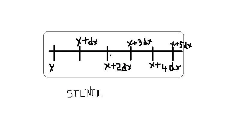
Skewed Right-sided difference is a finite difference method that optimises a approximation for differential operator at the first node,then the required nodes starting from the first on left-hand side and end on right-hand side

Deriving a fourth order approximation of second order derivative with assymetric stencil nodes by using taylor table method

`frac{d^2y}{dx^2}=a*f(x)+b*f(x+dx)+c*f(x+2*dx)+d*f(x+3*dx)+e*f(x+4*dx)+g*f(x+5*dx)`

	f(x)	`f'(x)*dx`	`f''(x)*dx^2`	`f'''(x)*dx^3`	`f''''(x)*dx^4`	`f'''''(x)*dx^5`
f(x)	a	0	0	0	0	0
f(x+dx)	b	b	`frac{b}{2}`	`frac{b}{6}`	`frac{b}{24}`	`frac{b}{120}`
f(x+2dx)	c	`2*c`	`frac{4*c}{2}`	`frac{8*c}{6}`	`frac{16*c}{24}`	`frac{32*c}{120}`
f(x+3dx)	d	`3*d`	`frac{9*d}{2}`	`frac{27*d}{6}`	`frac{81*d}{24}`	`frac{243*d}{120}`
f(x+4dx)	e	`4*e`	`frac{16*e}{2}`	`frac{64*e}{6}`	`frac{256*e}{24}`	`frac{1024*e}{120}`
f(x+5dx)	g	`5*g`	`frac{25*g}{2}`	`frac{125*g}{6}`	`frac{625*g}{24}`	`frac{3125*g}{120}`
	0	0	1	0	0	0

Matrix A is composed of transpose taylor table

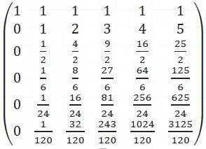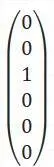A=,B=,X=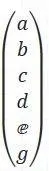

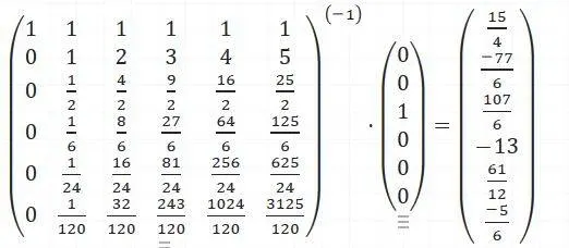
Matrix Inversion method `X=A^-1*B`

=

`frac{d^2y}{dx^2}=(0+frac{b}{2}+frac{4*c}{2}+frac{9*d}{2}+frac{16*e}{2}+frac{25*g}{2})*f''(x)*dx^2`

`frac{d^2y}{dx^2}=a*f(x)+b*f(x+dx)+c*f(x+2*dx)+d*f(x+3*dx)+e*f(x+4*dx)+g*f(x+5*dx)`

Substituting above equation on below equation to the matrix inversion method

`a*f(x)+b*f(x+dx)+c*f(x+2*dx)+d*f(x+3*dx)+e*f(x+4*dx)+g*f(x+5*dx)=(0+frac{b}{2}+frac{4*c}{2}+frac{9*d}{2}+frac{16*e}{2}+frac{25*g}{2})*f''(x)*dx^2`

Coefficient of Second order derivative is 1

`frac{d^2y}{dx^2}=frac{(frac{15}{4})*f(x)-(frac{77}{6})*f(x+dx)+(frac{107}{6})*f(x+2*dx)-13*f(x+3*dx)+(frac{61}{12})*f(x+4*dx)-(frac{5}{6})*f(x+5*dx)}{dx^2}`

Thumb Rule

Assymetric Scheme

No of nodes=6,Order of derivative=2

Order of accuracy (P)=6-2=4

Order of accuracy is 4

iii.Skewed left-sided difference

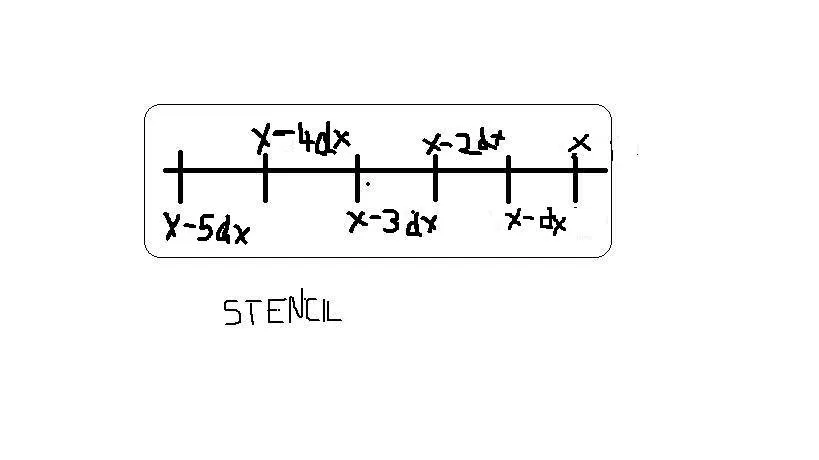
Skewed Right-sided difference is a finite difference method that optimises a approximation for differential operator at the first node,then the required nodes starting from the first on Right-hand side and end on left-hand side

Deriving a fourth order approximation of second order derivative with assymetric stencil nodes by using taylor table method

`frac{d^2y}{dx^2)=a*f(x)+b*f(x-dx)+c*f(x-2*dx)+d*f(x-3*dx)+e*f(x-4*dx)+g*f(x-5*dx)`

	f(x)	`f'(x)*dx`	`f''(x)*dx^2`	`f'''(x)*dx^3`	`f''''(x)*dx^4`	`f'''''(x)*dx^5`
f(x)	a	0	0	0	0	0
f(x-dx)	b	-b	`frac{b}{2}`	`frac{-b}{6}`	`frac{b}{24}`	`frac{-b}{120}`
f(x-2dx)	`c`	-2c	`frac{4*c}{2}`	`frac{-8*c}{6}`	`frac{16*c}{24}`	`frac{-32*c}{120}`
f(x-3dx)	`d`	`-3*d`	`frac{9*d}{2}`	`frac{-27*d}{6}`	`frac{81*d}{24}`	`frac{-243*d}{120}`
f(x-4dx)	`e`	`-4*e`	`frac{16*e}{2}`	`frac{-64*e}{6}`	`frac{256*e}{24}`	`frac{-1024*e}{120}`
f(x-5dx)	`g`	`-5*g`	`frac{25*g}{2}`	`frac{-125*g}{6}`	`frac{625*g}{24}`	`frac{-3125*g}{120}`
	0	0	1	0	0	0

Matrix A is composed of transpose taylor table

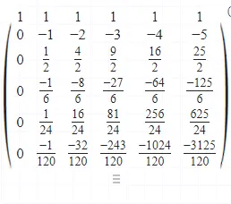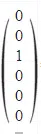A= ,B=,X=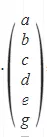

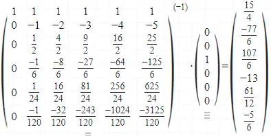
`X=A^-1*B`

=

`frac{d^2y}{dx^2}=a*f(x)+b*f(x-dx)+c*f(x-2*dx)+d*f(x-3*dx)+e*f(x-4*dx)+g*f(x-5*dx)`

`frac{d^2y}{dx^2}=(frac{1*b}{2}+frac{4*c}{2}+frac{9*d}{2}+frac{16*e}{2}+frac{25*g}{2})*frac{d^2y}{dx^2}*dx^2`

Substituting the above equation on next equation to matrix inversion method

`(frac{1*b}{2}+frac{4*c}{2}+frac{9*d}{2}+frac{16*e}{2}+frac{25*g}{2})*frac{d^2y}{dx^2}*dx^2=a*f(x)+b*f(x-dx)+c*f(x-2*dx)+d*f(x-3*dx)+e*f(x-4*dx)+g*f(x-5*dx)`

the coeffcient of second order derivative term is 1

`frac{d^2y}{dx^2}=frac{(frac{15}{4})*f(x)-(frac{77}{6})*f(x-dx)+(frac{107}{6})*f(x-2*dx)-13*f(x-3*dx)+(frac{61}{12})*f(x-4*dx)-(frac{5}{6})*f(x-5*dx)}{dx^2}`

Thumb Rule

Asymmetric Scheme

order of accuracy=no of nodes-Order of derivative

P=6-2=4

order of accuracy=4

Program

Main program

clc             %clear the command window
clear all       %clear all the workspace variables
close all       %close all the figure window

%inputs
i=1
x=pi/3
dx=linspace(pi/20,pi/1000,20)


for j=1:1:length(dx)
Exact_second_order_derivative=-2*exp(x)*sin(x);                  %second order derivative
[X]=central_differencing_scheme_Coefficients(5);                  %function call
%Central_differencing=(((-1/12)*f(x-2*dx))+((4/3)*f(x-dx))-((5/2)*f(x))+((4/3)*f(x+dx))-((1/12)*f(x+2*dx)))/(dx^2)
Central_differencing(j)=(((X(i))*f(x-2*dx(j)))+((X(i+1))*f(x-dx(j)))+((X(i+2))*f(x))+((X(i+3))*f(x+dx(j)))+((X(i+4))*f(x+2*dx(j))))/(dx(j)^2);
[X]=Skew_right_sided_coefficients(6);                             %function call
skew_right_sided_differencing(j)=(((X(i))*f(x))+((X(i+1))*f(x+dx(j)))+((X(i+2))*f(x+2*dx(j)))+((X(i+3))*f(x+3*dx(j)))+((X(i+4))*f(x+4*dx(j)))+(X(i+5)*f(x+5*dx(j))))/(dx(j)^2);
[X]=Skew_left_sided_coefficients(6);                           %function call
skew_left_sided_differencing(j)=(((X(i))*f(x))+((X(i+1))*f(x-dx(j)))+((X(i+2))*f(x-2*dx(j)))+((X(i+3))*f(x-3*dx(j)))+((X(i+4))*f(x-4*dx(j)))+(X(i+5)*f(x-5*dx(j))))/(dx(j)^2);
error_central_diff(j)=abs(Exact_second_order_derivative-Central_differencing(j));
error_skew_right_sided(j)=abs(Exact_second_order_derivative-skew_right_sided_differencing(j));
error_skew_left_sided(j)=abs(Exact_second_order_derivative-skew_left_sided_differencing(j));
end
%plots
figure(1)
loglog(dx,error_central_diff)
hold on
loglog(dx,error_skew_right_sided)
loglog(dx,error_skew_left_sided)
legend('Central difference','skew right sided scheme','skew left sided scheme')
xlabel('log(dx)')
ylabel('log(error)')
hold off

figure(2)
plot(dx,error_central_diff)
hold 
xlabel('dx')
ylabel('error')
plot(dx,error_skew_right_sided)
plot(dx,error_skew_left_sided)
legend('Central difference','skew right sided scheme','skew left sided scheme')
hold off

The function is used for calling an analtycal function

function var=f(x)
var=exp(x).*cos(x);        %analtycal function
end

Thess functions to calculate coefficients

function X=central_differencing_scheme_Coefficients(x)
if x==5
A=[1 1 1 1 1 ;-2 -1 0 1 2;4/2 1/2 0 1/2 4/2;-8/6 -1/6 0 1/6 8/6;16/24 1/24 0 1/24 16/24]  %taken from taylor table
B=[0;0;1;0;0]
X=inv(A)*B
end
end

function [X]=Skew_right_sided_coefficients(x)
if x==6
A=[1 1 1 1 1 1;0 1 2 3 4 5;0 1/2 4/2 9/2 16/2 25/2;0 1/6 8/6 27/6 64/6 125/6;0 1/24 16/24 81/24 256/24 625/24;0 1/120 32/120 243/120 1024/120 3125/120]
B=[0;0;1;0;0;0]
[X]=inv(A)*B
end
end

function [X]=Skew_left_sided_coefficients(x)
if x==6
A=[1 1 1 1 1 1;0 -1 -2 -3 -4 -5;0 1/2 4/2 9/2 16/2 25/2;0 -1/6 -8/6 -27/6 -64/6 -125/6;0 1/24 16/24 81/24 256/24 625/24;0 -1/120 -32/120 -243/120 -1024/120 -3125/120]
B=[0;0;1;0;0;0]
[X]=inv(A)*B
end
end

Plots

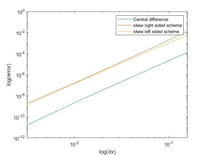
dx vs error

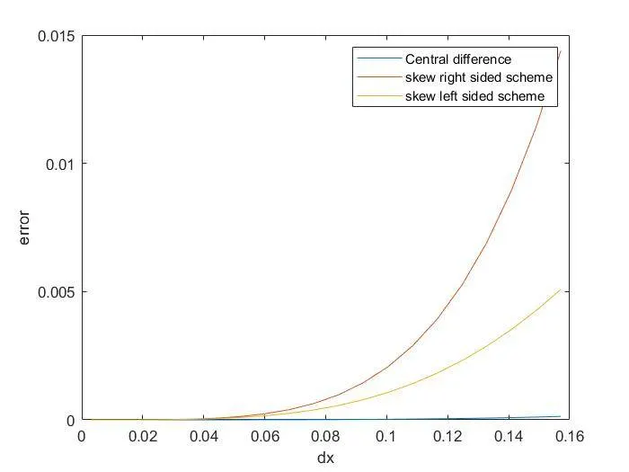
describe why a skewed scheme is useful? What can a skewed scheme do that a CD scheme cannot?

With the help of Skewed scheme,it can compute higher order derivative and higher order approximations for a one side stencil.CD scheme needs a symmetric stencil with a centre node that is a point need a derivative.Skewed scheme doesnot need a symmetric stencil.for example in a fluid flow domain at initial points and end points cannot able to use CD

Conclusion

Central Differencing Scheme have a high accuracy with low error compared to skewed left sided scheme and Skewed right sided scheme for a available symetric and asymetric stencil.Different schemes is available for different stencils.