Rankine cycle Simulator

Rankine Cycle

The Rankine cycle is a model used to predict the performance of steam turbine systems. It was also used to study the performance of reciprocating steam engines. The Rankine cycle is an idealized thermodynamic cycle of a heat engine that converts heat into mechanical work while undergoing phase change. It is an idealized cycle in which friction losses in each of the four components are neglected. The heat is supplied externally to a closed loop, which usually uses water as the working fluid. It is named after William John Macquorn Rankine, a Scottish polymath and Glasgow University professor.

• Process 1-2: The dry saturated vapour expands through a turbine, generating power. This decreases the temperature and pressure of the vapour, and some condensation may occur. The output in this process can be easily calculated using the chart or tables noted above.

In other words Process 1-2 is [Isentropic expansion]

• Process 2-3: The wet vapour then enters a condenser, where it is condensed at a constant pressure to become a saturated liquid.

In other words Process 2-3 is [Constant pressure heat rejection in condenser]

• Process 3–4: The working fluid is pumped from low to high pressure. As the fluid is a liquid at this stage, the pump requires little input energy.

In other words Process 3-4 is [Isentropic compression]

• Process 4-1: The high-pressure liquid enters a boiler, where it is heated at constant pressure by an external heat source to become a dry saturated vapour. The input energy required can be easily calculated graphically, using an enthalpy–entropy chart (h–s chart, or Mollier diagram), or numerically, using steam tables.

In other words Process 4-1 is [Constant pressure heat addition in boiler]

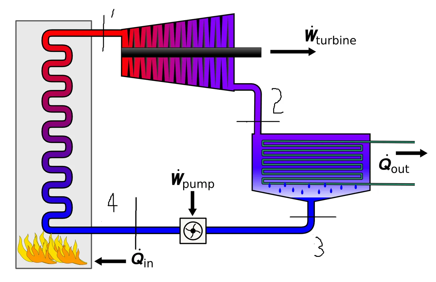
The traditional Rankine Cycle which uses water as the working fluid needs much higher temperature heat source while Organic Rankine Cycle (ORC) can generate power at a much lower temperature. The heat source temperature can vary from 50 to over 250°C.The working fluid for organic Rankine cycle is btane,pentane,hexane,silicon oil etc..

Efficiency of the Rankine Cycle=`frac{underset(Net)(W)}{underset(In)(Q)}`

`underset(Net)(W)` is total work developed by the rankine cycle

`underset(Net)(W)=underset(Turb)(W)-underset(Pump)(W)`

`underset(Turb)(W)=underset(1)(H)-underset(2)(H)`

`underset(1)(H)`=Enthalpy of the steam Exit from the boiler (taken from steam tables)

`underset(2)(H)=`Enthalpy of the steam Exit from the turbine (taken from steam tables)

`underset(Pump)(W)=underset(4)(H)-underset(3)(H)`

`underset(4)(H)=`Enthalpy of the liquid exit from the pump (taken from steam tables)

`underset(3)(H)=`Enthalpy of the liquid enter from the pump (taken from steam tables)

`underset(In)(Q)` is heat added in the 4-1 Process using a boiler

`underset(In)(Q)=underset(1)(H)-underset(4)(H)`

BackWork Ratio=`frac{underset(Pump)(W)}{underset(Turb)(W)}`

Specific Steam Consumption=`frac{3600}{underset(Net)(W)}`

Matlab Script

XSteam Function is used

clc
close all
clear all
format long
a='Rankine Cycle Simulator';                                                     
CmdWinSize = get(0, 'CommandWindowSize');                                     % Command used to get the length and width of the command window 
width=CmdWinSize(1);
b=length(a);
c='Results';
fprintf(blanks(floor((width-b)/2)));
fprintf('%sn',a);
fprintf('1-2 is Isentropic Expansion in the Turbine n');
fprintf('2-3 is Constant Pressure Heat Rejection by the condenser n');
fprintf('3-4 is Isentropic Compression in the Pump n');
fprintf('4-1 is Constant Pressure Heat Addition by the Boiler n');

%inputs
Press_in_state_1=input('Enter the Pressure at the Turbine Inlet (in bar):');
Temp_in_state_1=input('Enter the Temperature at the Turbine Inlet (in Degree celcius):');
Press_in_state_2=input('Enter the Pressure at the Condenser (in bar):');
fprintf(blanks(floor((width-length(c))/2)));
fprintf('%sn',c);
%%
%function call
Enthalpy_state_1=XSteam('h_pT',Press_in_state_1,Temp_in_state_1);
Entropy_state_1=XSteam('s_pT',Press_in_state_1,Temp_in_state_1);

%%
%entropy is constant for a Turbine
%State 2
Entropy_state_2=Entropy_state_1;
Sf2=XSteam('sL_p',Press_in_state_2);                                         %Entropy of the fluid for the pressure 
Sg2=XSteam('sV_p',Press_in_state_2);                                         %Entropy of the Gas for the pressure
Sfg2=Sg2-Sf2;
x=(Entropy_state_2-Sf2)/Sfg2;                                                %dryness fraction

hg2=XSteam('hV_p',Press_in_state_2);                                         %Enhalpy of the gas for the pressure using a Function call
                                                                             %Function XSteam
if(x<1)
    Temp_in_state_2=XSteam('Tsat_p',Press_in_state_2);
    hf2=XSteam('hL_p',Press_in_state_2);
    Enthalpy_state_2=hf2+(x*(hg2-hf2));
    
else
    term=exp((Entropy_state_2-Sg2)/XSteam('CpV_p',Press_in_state_2));        %https://www.grc.nasa.gov/www/k-12/VirtualAero/BottleRocket/airplane/entropy.html
  Temp_in_state_2_K=(XSteam('Tsat_p',Press_in_state_2)+273)*term;            %Saturated Temperature in kelvin
  Temp_in_state_2=Temp_in_state_2_K-273;
 Enthalpy_state_2=hg2+(XSteam('CpV_p',Press_in_state_2)*(Temp_in_state_2-XSteam('Tsat_p',Press_in_state_2)));
end
Work_done_Turbine=Enthalpy_state_1-Enthalpy_state_2;
%%
%State 3
Press_in_state_3=Press_in_state_2;
Temp_in_state_3=XSteam('Tsat_p',Press_in_state_3);
Enthalpy_state_3=XSteam('hL_p',Press_in_state_3);
Entropy_state_3=XSteam('sL_p',Press_in_state_3);

%%
%State 4
Entropy_state_4=Entropy_state_3;
Press_in_state_4=Press_in_state_1;

Volume_state_3=XSteam('vL_p',Press_in_state_3);
Work_Input_for_pump=Volume_state_3*(100*(Press_in_state_4-Press_in_state_3));  %converting the bar into kilo pascal by multiplying a 100
Enthalpy_state_4=Work_Input_for_pump+Enthalpy_state_3;
Work_net=Work_done_Turbine-Work_Input_for_pump;
Cp=XSteam('Cp_ph',Press_in_state_4,Enthalpy_state_4);                          %Specific heat for particular pressure and enthalpy
Cv=XSteam('Cv_ph',Press_in_state_4,Enthalpy_state_4);
gamma=Cp/Cv;
power=((gamma-1)/gamma);
P_ratio=((Press_in_state_3/Press_in_state_4)^power);
Temp_in_state_4=Temp_in_state_3/P_ratio;
Back_work_ratio=Work_Input_for_pump/Work_done_Turbine;
S_S_C=3600/Work_net;
Thermal_efficiency=Work_net/(Enthalpy_state_1-Enthalpy_state_4);

%%
%Print
fprintf('At State Point 1:         ') 
fprintf(blanks(floor((width-52))));                                            %Making a blank space inbetween the Print in the command window
fprintf('At State Point 4:         n')
fprintf(' P1 is :%4.2f Bar         ',Press_in_state_1)
fprintf(blanks(floor((width-52))));
fprintf('P4 is :%4.2f Bar         n',Press_in_state_4)
fprintf(' T1 is :%4.2f Deg celcius ',Temp_in_state_1)
fprintf(blanks(floor((width-53))));
fprintf('T4 is :%4.2fDeg celciusn',Temp_in_state_4)
fprintf(' H1 is :%4.2f kJ/Kg       ',Enthalpy_state_1)
fprintf(blanks(floor((width-55))));
fprintf(' H4 is :%4.2f kJ/Kg    n',Enthalpy_state_4)
fprintf(' S1 is :%4.2f kJ/Kg K     ',Entropy_state_1)
fprintf(blanks(floor((width-52))));
fprintf(' S4 is :%4.2f kJ/Kg K     nn',Entropy_state_4)

fprintf('At State Point 2:         ')
fprintf(blanks(floor((width-52))));
fprintf('Wt is :%4.2f kJ/kg       n',Work_done_Turbine)
fprintf(' P2 is :%4.2f Bar         ',Press_in_state_2)
fprintf(blanks(floor((width-52))));
fprintf(' Wp is :%4.2f kJ/kg       n',Work_Input_for_pump)
fprintf(' T2 is :%4.2f Deg celcius ',Temp_in_state_2)
fprintf(blanks(floor((width-52))));
fprintf('Wnet is :%4.2f kJ/Kg  n',Work_net)
fprintf(' H2 is :%4.2f kJ/Kg       ',Enthalpy_state_2)
fprintf(blanks(floor((width-54))));
fprintf('NTherm is :%3.3f%%n',Thermal_efficiency*100)
fprintf(' S2 is :%4.2f kJ/Kg K     ',Entropy_state_2)
fprintf(blanks(floor((width-52))));
fprintf(' S.S.C is :%f kg/KWh      n',S_S_C)
fprintf(' X is :%f ',x)
fprintf(blanks(floor((width-43))))
fprintf(' BackWork Ratio is :%f n',Back_work_ratio)

fprintf('At State Point 3:n')
fprintf(' P3 is :%f Barn',Press_in_state_3)
fprintf(' T3 is :%f Deg celciusn',Temp_in_state_3)
fprintf(' H3 is :%f kJ/Kgn',Enthalpy_state_3)
fprintf(' S3 is :%f kJ/Kg Kn',Entropy_state_3)


%%
%plot of T-s Diagram

Temperature=linspace(0.01,371.7,100);                                         %creating a row array for a temperature
for i=1:1:100
    Entropy_liquid_line(1,i)=XSteam('sL_T',Temperature(1,i));                 %creating a line in T-s Diagram for a liquid line using a function Xsteam
    Entropy_Gas_line(1,i)=XSteam('sV_T',Temperature(1,i));                    %creating a line in T-s Diagram for a Gas line using a function Xsteam
    Enthalpy_liquid_line(1,i)=XSteam('hL_T',Temperature(1,i));                %creating a line in H-s Diagram for a liquid line using a function Xsteam
    Enthalpy_Gas_line(1,i)=XSteam('hV_T',Temperature(1,i));                   %creating a line in H-s Diagram for a Gas line using a function Xsteam
end
Temperature_1=linspace(371.7,378.7,10);
Coeff_Entropy_liquid_line=polyfit(Temperature,Entropy_liquid_line,13);        %Determing a Equation to fill a bell shaped curve in T-s Diagram
Entropy_liquid_line_Curve_fit=polyval(Coeff_Entropy_liquid_line,Temperature_1);
Coeff_Entropy_Gas_line=polyfit(Temperature,Entropy_Gas_line,13);
Entropy_Gas_line_Curve_fit=polyval(Coeff_Entropy_Gas_line,Temperature_1);
Entropy_1=linspace(4,4.5,10);                                                 %Determing a Equation to fill a  curve in H-s Diagram
Coeff_Enthalpy_liquid_line=polyfit(Entropy_liquid_line,Enthalpy_liquid_line,13);
Enthalpy_liquid_line_Curve_fit=polyval(Coeff_Enthalpy_liquid_line,Entropy_1);
Entropy_2=linspace(4.5,5,10);
Coeff_Enthalpy_Gas_line=polyfit(Entropy_Gas_line,Enthalpy_Gas_line,13);
Enthalpy_Gas_line_Curve_fit=polyval(Coeff_Enthalpy_Gas_line,Entropy_2);
subplot(1,2,1)                                                                %On a one figure have two graphs on a one Row
plot(Entropy_liquid_line,Temperature,Entropy_liquid_line_Curve_fit,Temperature_1,Entropy_Gas_line_Curve_fit,Temperature_1,Entropy_Gas_line,Temperature,'color',[1 0 0])
hold on
K=plot([Entropy_state_1 Entropy_state_2],[Temp_in_state_1 Temp_in_state_2] );
M=plot([Entropy_state_3 Entropy_state_4],[Temp_in_state_3 Temp_in_state_4] );
O=plot([XSteam('sL_p',Press_in_state_4) XSteam('sV_p',Press_in_state_4)],[XSteam('Tsat_p',Press_in_state_4) XSteam('Tsat_p',Press_in_state_4)] );
P=plot([XSteam('sV_p',Press_in_state_4) Entropy_state_1 ],[XSteam('Tsat_p',Press_in_state_4) Temp_in_state_1] );
Q=plot([XSteam('sL_p',Press_in_state_4) Entropy_state_4 ],[XSteam('Tsat_p',Press_in_state_4) Temp_in_state_4] );

if x>1
L=plot([Entropy_state_3 XSteam('sV_T',Temp_in_state_3)],[Temp_in_state_3 Temp_in_state_3] );
N=plot([XSteam('sV_T',Temp_in_state_3) Entropy_state_2],[Temp_in_state_3 Temp_in_state_2] );
A=[K L M N O P Q];
else
   L=plot([Entropy_state_3 Entropy_state_2],[Temp_in_state_3 Temp_in_state_2] );
   A=[K L M O P Q];
end

set(A,'color','b','LineWidth',1)                                              %Command used to set a colour and linewidth
text(Entropy_state_1+0.2,Temp_in_state_1+0.1,'1');
text(Entropy_state_2+0.2,Temp_in_state_2+0.1,'2');
text(Entropy_state_3+0.2,Temp_in_state_3+0.1,'3');
text(Entropy_state_4+0.2,Temp_in_state_4+0.1,'4');
xlabel('Entropy in kJ/kg K')
ylabel('Temperature in  C')
title('TS Diagram')
grid on
hold off
%plot of h-s diagram
subplot(1,2,2)
plot(Entropy_liquid_line,Enthalpy_liquid_line,Entropy_Gas_line,Enthalpy_Gas_line,Entropy_1,Enthalpy_liquid_line_Curve_fit,Entropy_2,Enthalpy_Gas_line_Curve_fit,'color',[1 0 0])
hold on
J=plot([Entropy_state_1 Entropy_state_2],[Enthalpy_state_1 Enthalpy_state_2],[Entropy_state_2 Entropy_state_3],[Enthalpy_state_2 Enthalpy_state_3],[Entropy_state_3 Entropy_state_4],[Enthalpy_state_3 Enthalpy_state_4],[Entropy_state_4 Entropy_state_1],[Enthalpy_state_4 Enthalpy_state_1] );
set(J,'color','b','LineWidth',1)
text(Entropy_state_1+0.2,Enthalpy_state_1+0.1,'1');
text(Entropy_state_2+0.2,Enthalpy_state_2+0.1,'2');
text(Entropy_state_3+0.2,Enthalpy_state_3+0.1,'3');
text(Entropy_state_4+0.2,Enthalpy_state_4+0.1,'4');
xlabel('Entropy in kJ/kg K')
ylabel('Enthalpy in  kJ/kg')
title('HS Diagram')
grid on
hold off

Code Explanation

clc,close all,clear all is used to clear the command window and close all the figure window and clear all the workspace variables

Get command is used to get the length and width of the command window

Blanks on the fprintf command is used to leave a space on command window to display at the centre

floor command is used to round off the value and fprintf is used to display the process in commnad window

Input command is assigned to the three variables to get three inputs

Under the Function call comment,XSteam is used,it is function

there made a function call by specify a inputs and to get the values for different paramaters

If condition is used by specifying a condition X<1 executes a True or false block with the help of condition

Under the print comment used a Fprintf command to display a statements

Using blank command leave a space between two statements

Polyfit command is used to find a equation for the available data

polyval command is used to find a values using a determined coefficients,x values

set command is used to assign a properties for a plot

Text command is used to mention the string at a described dimensions

Xlabel command is used to mention the string on the X-axis

Ylabel command is used to mention the string on the Y-axis

title command is used to mention the name of the Graph using a String

Output

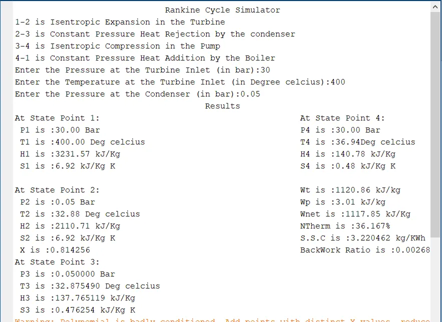
Plot

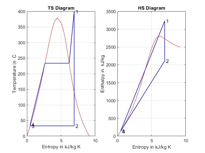
Conclusion

Thus, can calculate a Thermal efficiency,Specific Steam Consumption,Back work Ratio and T-S,H-s graphs for different inputs