Week 8- Moving zones approach in Fluent

Introduction:

• Stationary (or inertial) Reference Frame: Ansys Fluent solves the equation of the heat transfer and fluid flow, by default, in a stationary reference frame. However, there are many problems where it is advantageous to solve equations in a moving(non-inertial) reference frame. such problem typically involves moving parts such as rotating blades, impellers etc.
• in most cases, moving parts render the problem unsteady when viewed from the stationary frame. however, the flow around the moving parts can be modelled as steady with respect to the moving reference frame.

Question 1: What are the approaches by which you would model the moving zone?

Answer 1: Introduction to moving zone:

• Two types of motion are involved in the fluid flow problem
  1. Rectilinear
  2. Rotary

• To model rotary motion, two approaches are used
  1. Moving Reference Frame (MRF)
  2. Moving Mesh Method (MMM)

1. Moving Reference Frame (MRF): it describes the use of a single moving reference frame, multiple moving reference frames, and mixing planes in Ansys Fluent. MRF approach is a steady-state method employed in industrial computational fluid dynamics to model problems with rotating parts.
   • Single reference frame: Refer the entire computational domain to a single moving reference frame approach.
   • Multiple reference frame: In complex geometry, it is not possible to use a single reference frame. In such cases breakup the problem into multiple cell zones with well-defined interfaces between the cell zones.

In Ansys Fluent, by enabling the moving reference frame in selected cell zones, we can model the problem involving moving parts. when the moving reference frame is activated, equations of motion are modified by incorporating the additional acceleration term due to the transformation stationary reference frame to a moving reference frame. By solving these equations in a steady state manner, the flow around the moving parts can be modelled.

Circular interface:

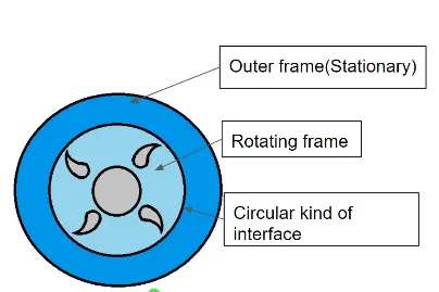
Figure: Circular interface

• The Navier-stoke equation in a stationary frame is solved separately
• Navier-stoke equation in moving frame is solved separately
• data is transferred from one frame to another frame through the interface by using following methods
  • Area averaging
  • Mass averaging
  • Mixed-out approach (best method because of no averaging)
    • Solve the following equations
      1. X-Momentum
      2. Y-Momentum
      3. Z-Momentum
      4. Energy

Question 2: Which approach would you use to model the unsteady phenomenon?

Answer 2: Moving Mesh Method (MMM): It describes the sliding and deforming mesh in Ansys Fluent. MMM are adaptive techniques for solving partial differential equations where the grid involves to improve the approximation to the solution.

• Sliding mesh method: If unsteady interaction between stationary and moving part is important then employ the sliding mesh method to capture the transient behaviour of fluid flow.

S.No.	Moving Reference Frame (MRF)	Moving Mesh Method (MMM)
1.	Frame is moving	Mesh is moving
2.	Steady phenomenon if unsteadiness is not important	Unsteady phenomenon if unsteadiness is important
3.	No change in the control volume	Control volume changes with time
4.	Mesh topology remains same	Topology changes with time

Question 3: Simulate rotary motion for the geometry given

Answer: To model a problem involving a single moving reference frame, follow the steps outlined below

Step 1:

• The pressure-Based solver can use either absolute velocity formulation or relative velocity formulation
  • Choosing the Absolute or Relative velocity formulation
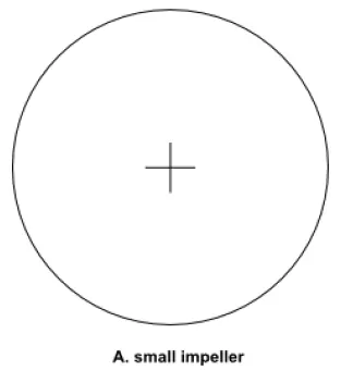
    • Absolute velocity formulation is preferred where the flow in the domain is not moving
      • Example: Small impeller in which flow near the impeller would be rotating and away from the impeller would be low velocity magnitude.
      • 
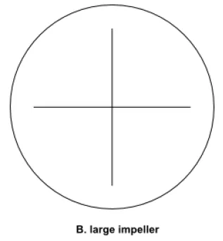
    • Relative velocity formulation is preferred where most of the fluid in a domain is moving
      • Example: large impeller in which flow is expected to be rotating with a velocity close to impeller.
      • 
• Density-Based Solver always use absolute velocity formulation. Relative velocity formation is not available in density based solver.

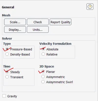
Figure: Setup

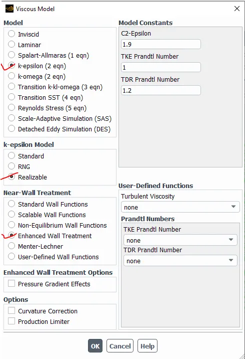
Figure: Viscous model

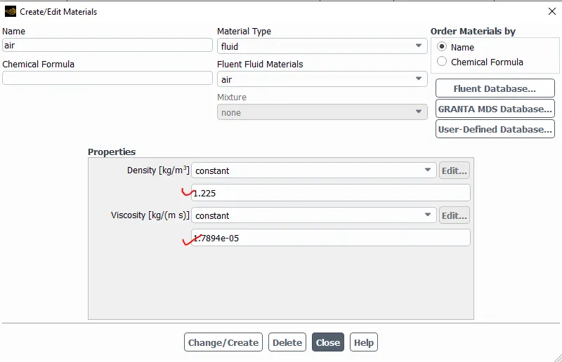
Figure: Material properties of air

Step 2:

• For each cell zone in the domain, specify the translational velocity of the reference frame and/or the angular velocity of the reference frame and the axis about which it rotates. here the frame is rotating at 250 rpm speed.

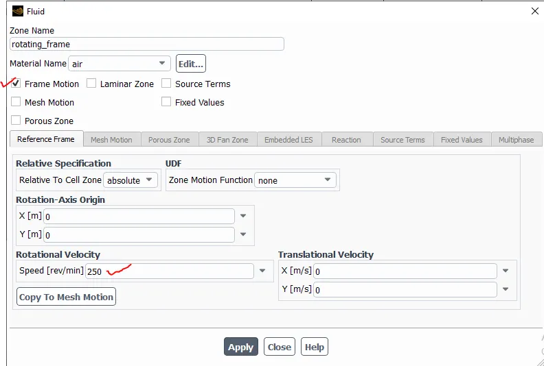
Figure: Cell zone condition

Step 3: Defining the velocity boundary conditions at walls. we can choose either an absolute velocity or a velocity relative to the moving reference frame (that is, relative to the velocity of the adjacent cell zone. Here the wall is moving at a speed of 250 rpm which is equal to the rotating frame (i.e. Adjacent cell zone). therefore, Relative angular velocity will be zero.

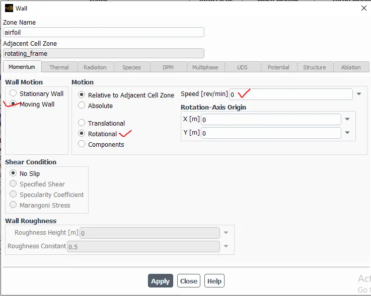
Figure: Wall boundary condition of the airfoil

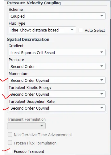
Figure: Solution method

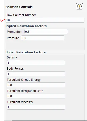
Figure: Solution control

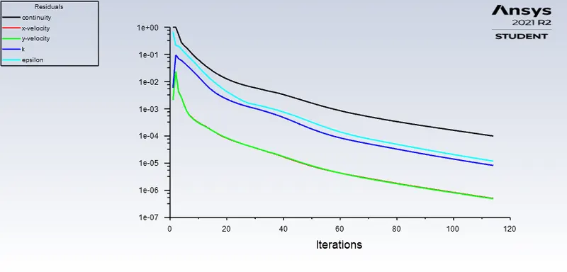
Figure: Residuals

The absolute criteria of residuals are set to 0.0001 in the residual monitors. and the solution is converged at 114 iterations. where the residual of continuity, x-velocity, y-velocity, turbulence kinetic energy(k) and dissipation rate of turbulent kinetic energy(`epsilon`) are shown in the given screenshot which meets the criteria (1e-04).

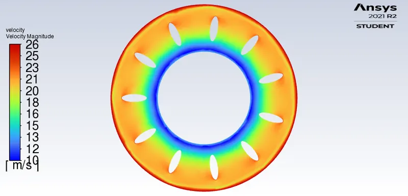
Figure: Velocity vector

The conclusion from the velocity vector:

maximum velocity (26 m/s) is at rotating domain_outer and minimum velocity (10 m/s) is at rotating domain_inner.