Week - 8 Mass Scaling
Week - 8 Mass Scaling
Aim
To reduce the runtime of a model using mass scaling while ensuring stability, with a hard limit of 8% on mass scaling. The objective is to achieve identical behaviour in simulations with and without mass scaling, optimize the DT and TSSFAC parameters, and compare the performance of explicit and implicit solvers.
Output Required
The following deliveries are needed from the simulation:
1. Mass Scaling Trials:
- Conduct multiple trials with varying mass scaling percentages up to 8%.
- Optimize DT and TSSFAC parameters for each trial.
- Ensure stability and identical behaviour in simulations with and without mass scaling
2. Data Generation:
- Collect and document data from each mass scaling trial.
- Record runtime, stability metrics, and any deviations in behaviour.
3. Histogram Plot:
- Create a histogram comparing the model's runtime across different mass scaling trials.
- Highlight the optimal mass scaling percentage that achieves the desired runtime reduction and stability.
4. Implicit Solver Comparison:
- Run the same model using an implicit solver with necessary adjustments.
- Compare the runtime and performance of the implicit solver against the explicit solver with mass scaling.
5. Final Report:
- Compile all findings, including mass scaling trials, data, histogram, and solver comparison.
- Provide a detailed analysis of the impact of mass scaling on runtime and stability.
- Discuss the advantages and limitations of using mass scaling and implicit solvers in simulations.
Introduction
In explicit methods, the time step is typically very small to ensure numerical stability. However, this small step size can hinder the method's utility for routine analysis. To mitigate CPU costs and enhance performance, mass scaling is commonly employed to augment the time step size of each cycle. LSDYNA offers several approaches for this purpose. One straightforward method involves using a higher mass density for the blank. Alternatively, users can define a minimum time step size in *CONTROL_TIMESTEP.
Excessively increasing the mass may lead to significant penetration issues and amplify dynamic effects, potentially rendering the results unusable. Therefore, monitoring penetrations and kinetic energy is crucial for obtaining reliable outcomes.
1. What is Mass Scaling
Mass scaling refers to a technique whereby nonphysical mass is added to a structure to achieve a larger explicit timestep.
Adding nonphysical mass to increase the timestep in a dynamic analysis invariably influences the results, as per the equation F=m*a. Often, this impact is negligible, and in such instances, the addition of nonphysical mass can be justified. This may apply when mass is added to a few minor elements in an area of low concern, or in quasi-static simulations where the velocity is minimal, and the kinetic energy is trivial compared to the peak internal energy. Ultimately, it is the analyst's responsibility to assess the impact of mass scaling. It may be necessary to lessen or remove mass scaling in subsequent runs to determine the results' sensitivity to the added mass.
1. What is Mass Scaling
Mass scaling refers to a technique whereby nonphysical mass is added to a structure to achieve a larger explicit timestep.
Adding nonphysical mass to increase the timestep in a dynamic analysis invariably influences the results, as per the equation F=m*a. Often, this impact is negligible, and in such instances, the addition of nonphysical mass can be justified. This may apply when mass is added to a few minor elements in an area of low concern, or in quasi-static simulations where the velocity is minimal, and the kinetic energy is trivial compared to the peak internal energy. Ultimately, it is the analyst's responsibility to assess the impact of mass scaling. It may be necessary to lessen or remove mass scaling in subsequent runs to determine the results' sensitivity to the added mass.
2. Types Of Mass Scaling
Mass scaling in LS-DYNA can be categorized into two main types: manual mass scaling and automatic mass scaling.
a. Manual Mass Scaling
Manual mass scaling in LS-DYNA involves selectively increasing the material density of specific parts in a model to achieve a larger explicit time step, thereby reducing computational cost and improving performance. This method is controlled by the user and is done independently of automatic mass scaling. While it can enhance simulation efficiency, adding nonphysical mass can affect the results, so it’s crucial to assess the sensitivity of the outcomes to the amount of mass added. This technique is beneficial in quasi-static simulations where the velocity is low, and the kinetic energy is minimal compared to the peak internal energy. Adjusting parameters like TSSFAC can further improve stability when using manual mass scaling.
b. Automatic Mass Scaling
Automatic mass scaling is a technique used in finite element analysis (FEA) to adjust the mass of elements in a model to achieve a desired time step size. This is particularly useful in explicit dynamic simulations, such as crash analysis, where the time step size is critical for stability and accuracy.
The primary goal of automatic mass scaling is to increase the time step size without compromising the accuracy of the simulation. This is achieved by artificially increasing the mass of certain elements, increasing the time step size.
How It Works
- Time Step Calculation: In explicit simulations, the model's smallest element dictates the time step size. Smaller elements result in reduced time steps, leading to a substantial increase in computational time.
- Mass Adjustment: To counteract this, automatic mass scaling is employed to augment the time step size by slightly increasing the mass of these small elements. This increment in mass enhances their characteristic length, thereby enlarging the time step size.
- Control Parameters: Users can manage the degree of mass scaling by setting parameters like the desired time step size and the maximum permissible mass addition. This control helps prevent the mass scaling from significantly altering the model's physical behaviour.
Benefits
- Reduced Computation Time: By increasing the time step size, automatic mass scaling can significantly reduce the overall computation time of the simulation.
- Improved Stability: It helps in maintaining the stability of the simulation, especially in cases where very small elements are present.
Considerations
- Accuracy: While automatic mass scaling can improve computational efficiency, it is essential to monitor the impact on the accuracy of the results. Excessive mass scaling can lead to unrealistic results.
- Application: It is most beneficial in simulations where small elements are necessary for capturing detailed geometry or localized phenomena but would otherwise lead to prohibitively small time steps.
In LS-DYNA, automatic mass scaling can be controlled using specific keywords and parameters, allowing users to fine-tune the balance between computational efficiency and accuracy.
Implementing Automatic Mass Scaling in LS-DYNA
In LS-DYNA, automatic mass scaling is controlled using specific keywords. The primary keyword for mass scaling is CONTROL_TIMESTEP and it has the following parameters.
- DT2MS: Target time step size for mass scaling.
- DT2MSF: Factor for mass scaling. If set to a value greater than 1, mass scaling is applied.
- TSSFAC: Scale factor for the stable time step size.
- DTINIT: Initial time step size.
- DTMIN: Minimum time step size allowed.
To implement mass scaling effectively, start by identifying the elements in your model causing the smallest time steps, as these will be most affected by mass scaling. Set an appropriate target time step size based on your simulation requirements. Adjust the mass scaling factor, beginning with a small factor and gradually increasing it if necessary. Run the simulation and monitor the results to ensure stability and accuracy, sure that mass scaling does not adversely affect the outcomes. Fine-tune the parameters to balance computational efficiency and accuracy. Best practices include making incremental adjustments to the mass scaling factor to avoid significant errors, validating the simulation results with and without mass scaling to ensure physical behaviour remains consistent, and documenting all parameters and results for future reference and reproducibility. By carefully implementing and monitoring automatic mass scaling, you can achieve a more efficient and stable simulation without compromising accuracy.
CONTROL_TIMESTEP Card
The CONTROL_TIMESTEP card controls the time step size in explicit simulations. The time step size is critical for the stability and accuracy of the simulation. In explicit dynamics, the time step size is typically too small to ensure numerical stability, especially when dealing with high-speed events like crash simulations.
The parameters and their values include,
1. DT2MS:
- The target time step size is set for mass scaling.
- Its role is to define the preferred time step size. Mass scaling will occur to augment the time step size if it falls below this target value.
- The typical value varies based on the simulation's unique needs. For instance, a common value might be 1e-6 seconds.
2. DT2MSF:
- The factor for mass scaling defines the degree to which mass scaling is applied.
- A value exceeding 1 signifies the activation of mass scaling.
- The standard value is 1.0, which indicates that mass scaling is in effect.
3. TSSFAC:
- The scale factor is applied to the stable time step size.
- Its role is to multiply the calculated stable time step size, ensuring a safety margin.
- The typical value is 0.9, which offers a 10% safety margin.
4. DTINIT:
- Initial Time Step Size.
- The purpose is to establish the initial time step size at the start of the simulation.
- The typical value is comparable to DT2MS, for instance, 1e-6 seconds.
5. DTMIN:
- The minimum allowable time step size prevents the time step from dropping below a specified limit, which could result in an unreasonable computation time.
- The typical value is set extremely low, for instance, 1e-8 seconds.
Procedure
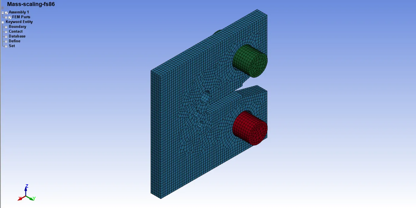
Step 01: Importing And Inspecting The Model
Download the keyword file and save it in a suitable location. Open LS-Prepost and load the keyword file (.K format). Open the keyword manager and understand the model with the assistance of the keyword manager.
Step 02: Running The Simulation With DT2MS = -3.5e-5 and TSSFAC = 0.9 (Default)
Initially, define a CONTROL_TIMESTEP card with default values for DT2MS and TSSFAC, and set the initial timestep value on the card.
- DT2MS = -3.5e-5
- TSSFAC = 0.9
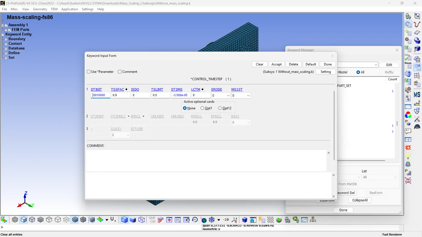
Then run the simulation, and inspect the running time and the added mass value.
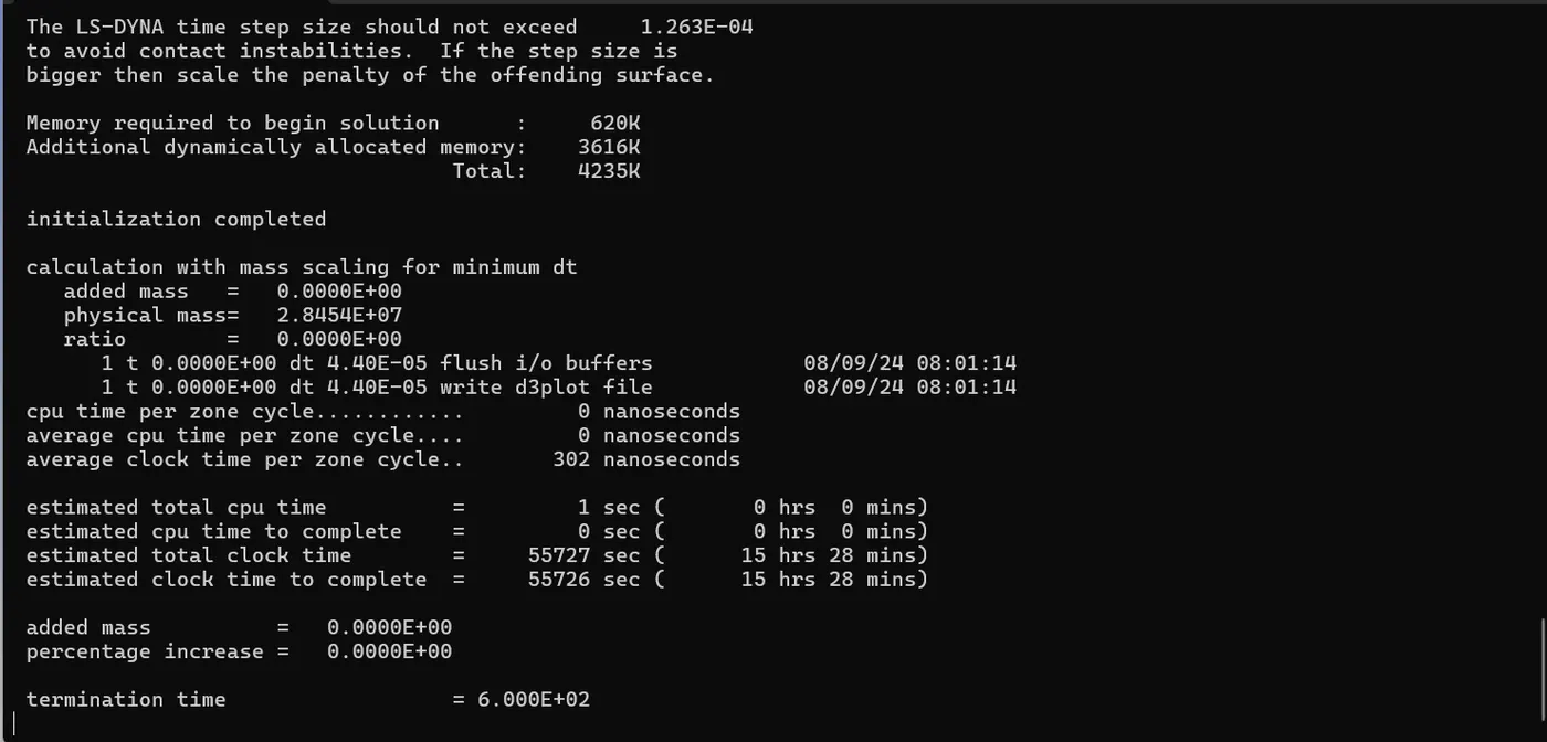
The message above indicates the values for 'estimated total clock time' and 'added mass'.
- Estimated Total Clock Time = 15 hrs and 28 mins
- Added Mass = 0.000e0
- Percentage Increase = 0.000e0
Step 03: Running The Simulation With DT2MS = -3.0e-5 and TSSFAC = 0.9
Define a CONTROL_TIMESTEP card with default values for DT2MS and TSSFAC, and set the initial timestep value on the card.
- DT2MS = -3.0e-5
- TSSFAC = 0.9
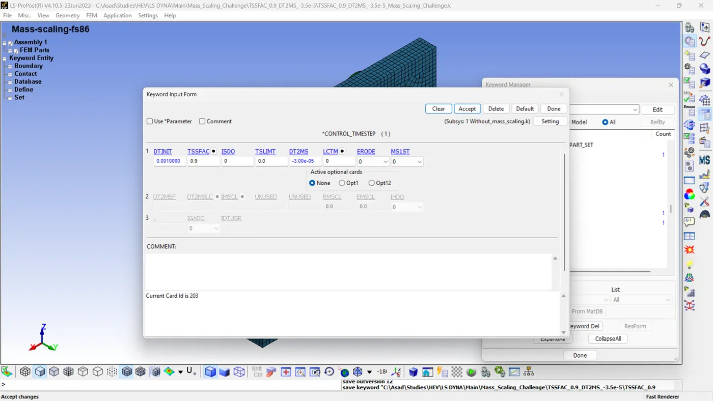
Next, execute the simulation and examine both the running time and the value of the added mass.
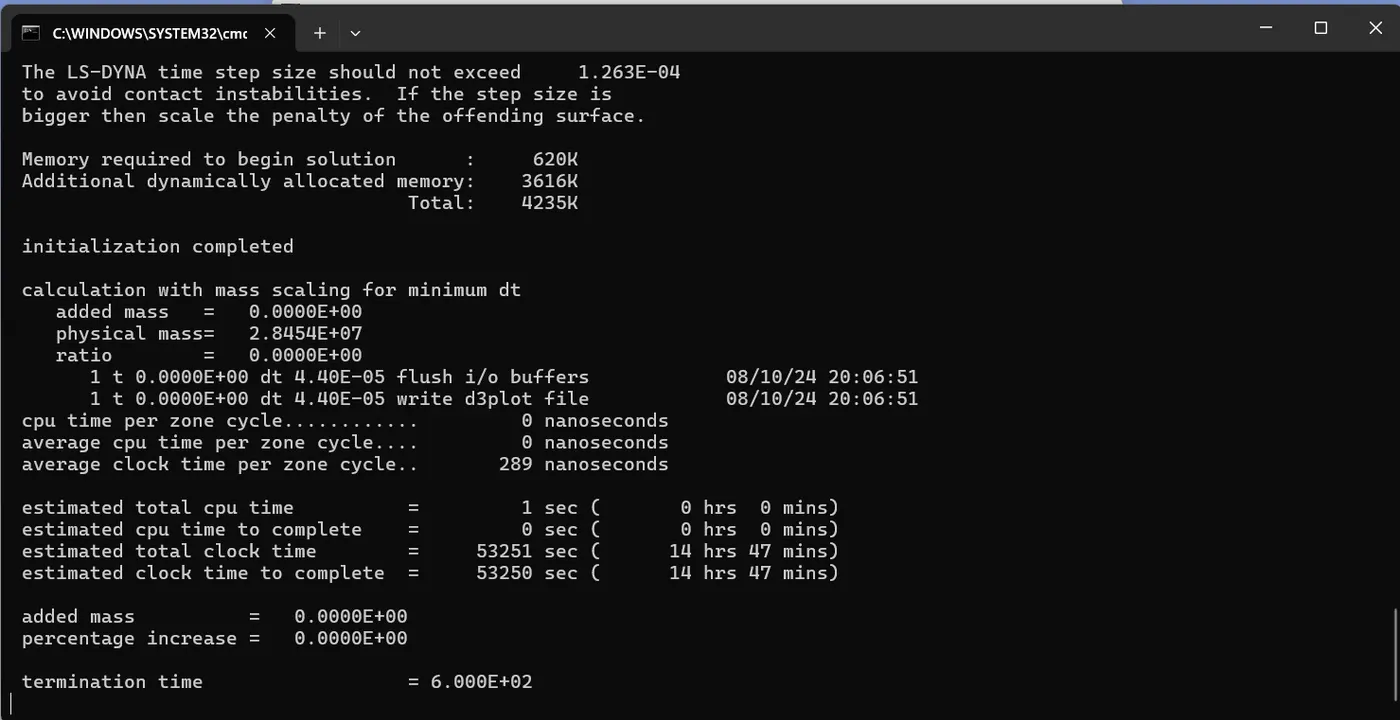
The message above indicates the values for 'estimated total clock time' and 'added mass'.
- Estimated Total Clock Time = 14 hrs and 47 mins
- Added Mass = 0.000e0
- Percentage Increase = 0.000e0
Step 04: Running The Simulation With Different Values of DT2MS and TSSFAC = 0.9
Similarly, we need to simulate the model with Different Values of DT2MS and TSSFAC = 0.9 and then tabulate the values. The goal is to determine the value of DT2MS, which is expected to show an approximate 8% increase in percentage.
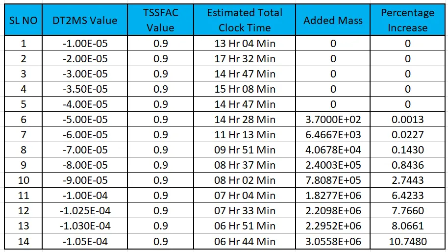
At DT2MS = -10.3E-5 and TSSFAC = 0.9 we can get a percentage mass increase of 8.0661%
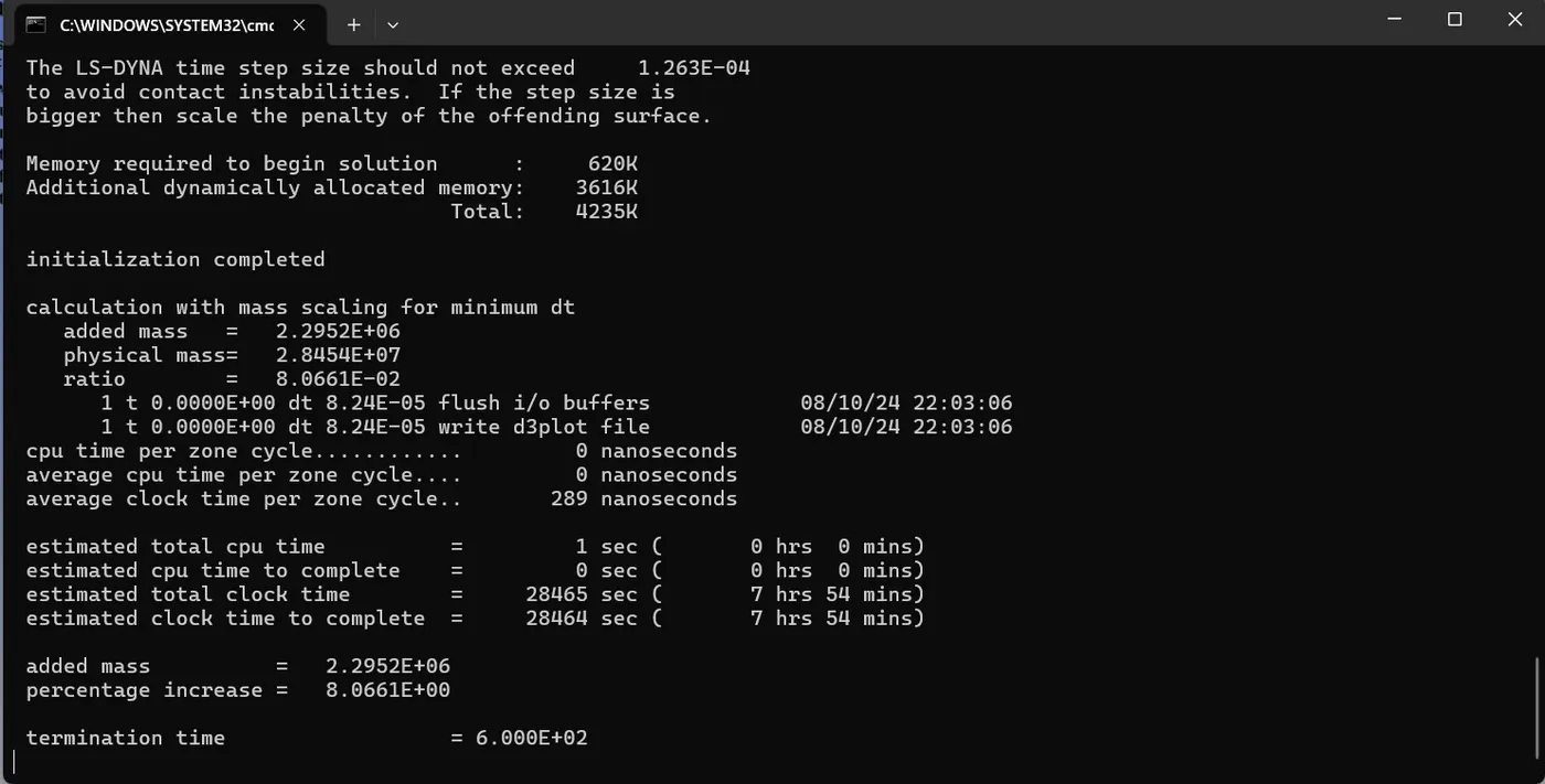
- Estimated Total Clock Time = 06 hrs and 51 mins
- Added Mass = 2.2952E06
- Percentage Increase = 8.0661
Step 05: Running The Simulation With Different Values of TSSFAC and DT2MS = -10.3E-5
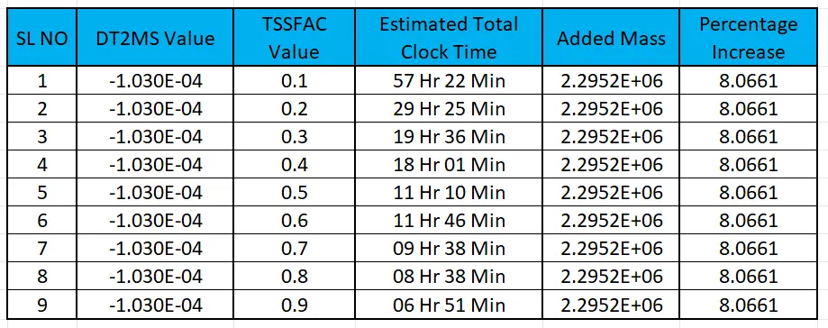
From the information provided, we have determined a DT2MS value that results in an 8% increase in mass percentage. Next, we must adjust the TSSFAC value to examine the impact of TSSFAC values on mass scaling.
Step 06: Running The Simulation Using Implicit Analysis
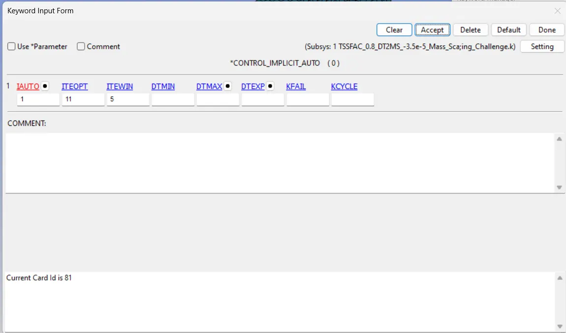
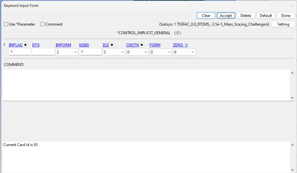
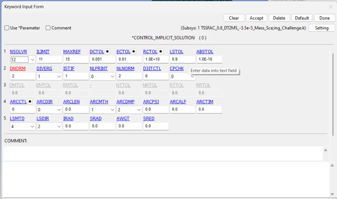
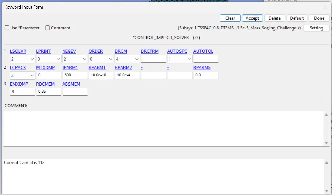
Defining the implicit control cards outlined below is necessary to perform an implicit method with suitable parameters.
1. CONTROL_IMPLICIT_AUTO
2. CONTROL_IMPLICIT_GENERAL
3. CONTROL_IMPLICIT_SOLUTION
4. CONTROL_IMPLICIT_SOLVER
Then, run the simulation and inspect the message.
Results
1. Changing DT2MS Values
The histograms below represent the outcomes of simulations in which the DT2MS values were varied for each run.
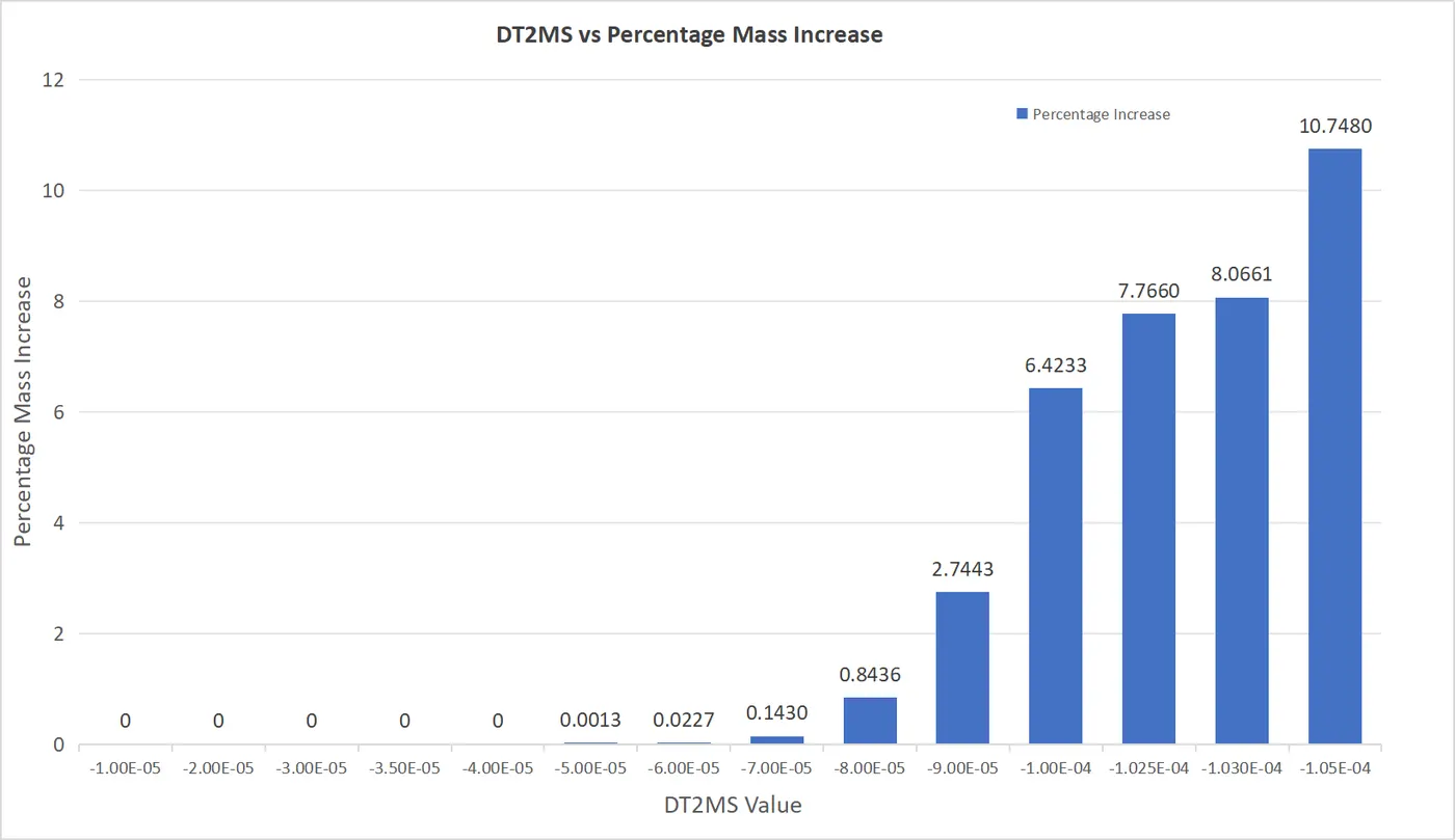
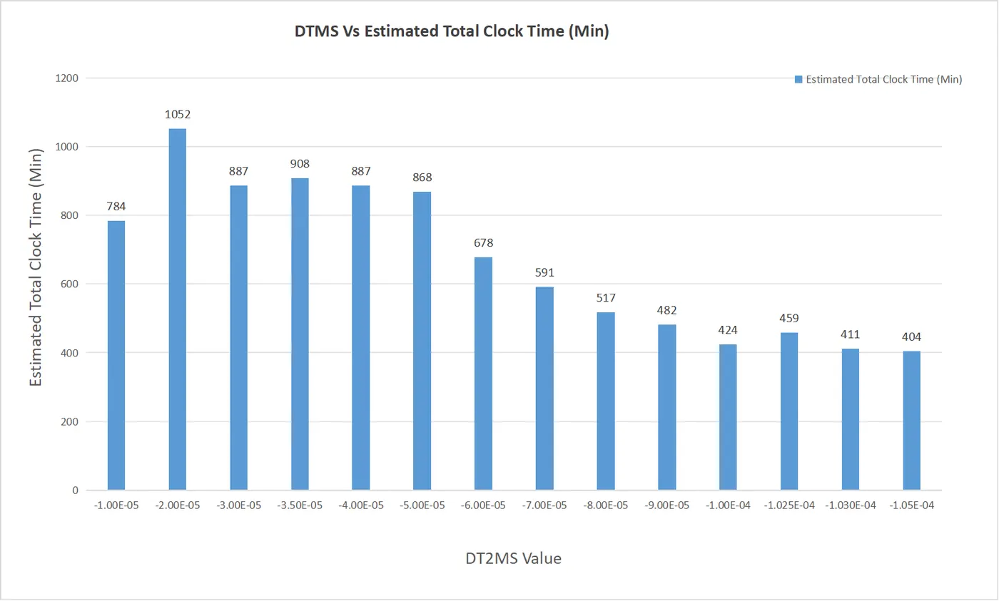
- When the DT2MS value falls within the range of -1E-05 to -5E-05, it indicates that no mass has been added to the simulation to allow for a larger time step. Furthermore, the estimated simulation time for these DT2MS values typically ranges between 13 and 18 hours.
- After setting DT2MS to -5E-05, an additional 0.0013% of the total mass is introduced to the system. As the DT2MS value is increased from -5E-05, the estimated simulation time starts to decline. Each decrement of DT2MS by -1E-05 results in a significant increase in the system's mass, thereby reducing the estimated simulation time from 11 to 6 hours.
- After increasing the DT2MS value from -1E-04 to -1.05E-04, the percentage mass increase surged to 10.784% from 6.4233%. However, our objective is to optimize the simulation so that the mass increases by exactly 8%. Following the initial setting of DT2MS at -1E-04, we decreased the increment of DT2MS and ultimately achieved a mass increase of 8.0661% at DT2MS = -1.030E-04. The estimated simulation time for this DT2MS value is 6 hours and 51 minutes.
2. Changing TSSFAC Values
From the trials mentioned, we obtained a DT2MS value of 1.030E-04, resulting in a mass increase of 8.0661%. The TSSFAC value used in that simulation was 0.9, which is considered ideal. We will now vary the TSSFAC value from 0.1 to 0.9 for the same DT2MS value and analyze the outcomes.
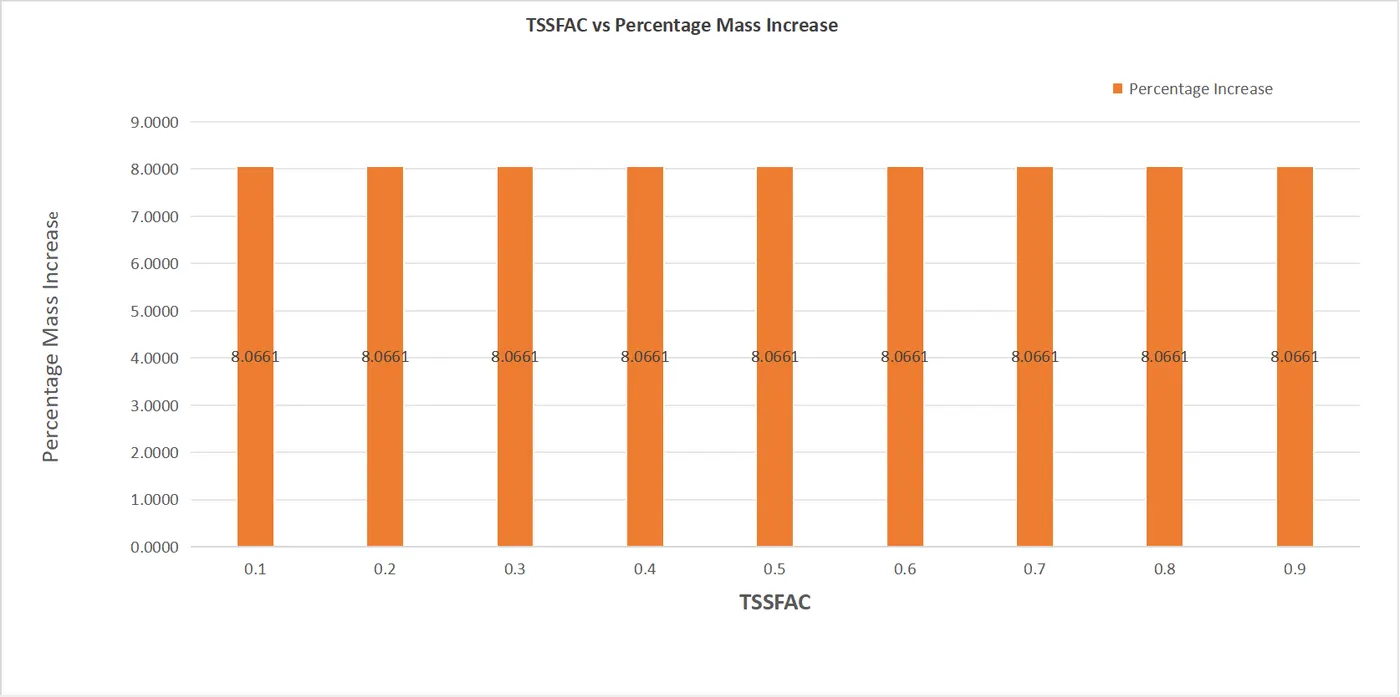
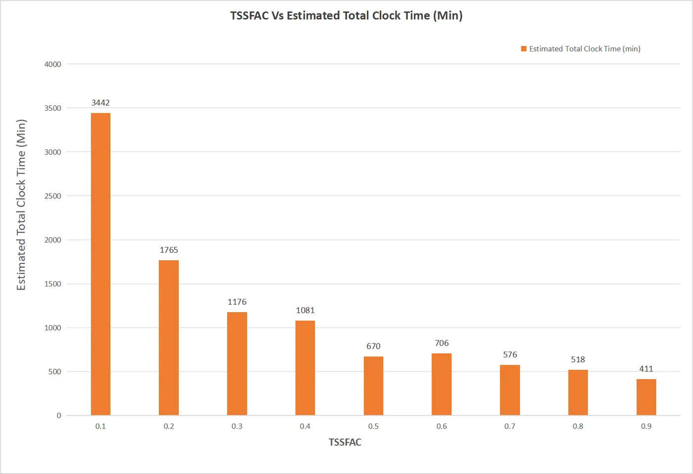
- It appears that alterations in TSSFAC values do not influence the percentage increase in mass. The percentage increase in mass remains 8.0661% when we change the TSSFAC value from 09 to 0.1 for the same DT2MS=-1.030E-04.
- The Time Step Scale Factor (TSSFAC) significantly impacts the estimated simulation time. Decreasing the TSSFAC value in increments of 0.1 from 0.9 to 0.1 results in a sharp increase in simulation time. At a TSSFAC value of 0.1, the simulation time soars to 57 hours and 27 minutes.
3. Implicit Analysis
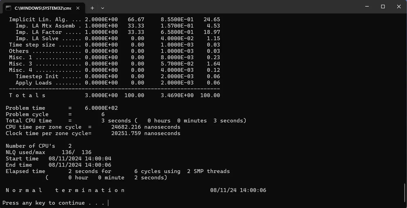
From the implicit method, the problem is solved in 2 seconds is much less than in explicit analysis. Implicit methods, in contrast, involve solving a system of equations that includes both the current and future states, typically using iterative solvers. These methods are unconditionally stable, which permits larger time steps without sacrificing stability. However, each step requires significant computational resources. This approach can decrease the total runtime for static or quasi-static problems, like structural analysis with constant loads, where the primary concern is determining equilibrium states.
In implicit analysis, mass scaling is generally less relevant compared to explicit analysis. This is because implicit methods are unconditionally stable and can handle larger time steps without compromising stability. However, mass scaling can still be applied in implicit analysis to improve computational efficiency, especially in quasi-static simulations.
Conclusion
- As per the objective, the ideal value of DT2MS and TSSFAC will be
DT2MS = -1.030E-04
TSSFAC = 0.9
Percentage Mass Increase = 8.0661
Estimated Simulation Time = 6Hr 51 Min - The parameter DT2MS is used for mass scaling, which can significantly affect simulation time. When set to a negative value, DT2MS adds mass to elements with time steps smaller than the absolute value of DT2MS, effectively increasing their time step. This reduces the total number of time steps required, thereby decreasing overall simulation time and improving computational efficiency. However, while mass scaling speeds up simulations, it can introduce nonphysical effects due to the added mass, especially in dynamic simulations where inertia forces are significant. Therefore, careful application and validation are necessary to ensure accuracy. In dynamic simulations, mass scaling helps overcome small time steps dictated by stability criteria, while in quasi-static problems, it can be applied more liberally without severely impacting accuracy.
- The TSSFAC parameter, short for the time step scale factor, is pivotal in controlling simulation duration by modifying the time step size. Defaulting to 0.9, a lower TSSFAC bolsters stability but at the expense of increased computational time due to finer time steps. On the flip side, a higher TSSFAC permits broader time steps, cutting down the simulation time, yet potentially undermining stability. Thus, judicious tuning of TSSFAC is essential to strike a balance between simulation duration and stability, ensuring time steps are neither excessively small, leading to high computational costs, nor excessively large, posing a risk of instability. Notably, TSSFAC's primary role is to adjust time step size in simulations without directly impacting mass scaling. TSSFAC adjusts the overall time step size to enhance stability or efficiency, it does not alter the amount of mass added to elements
- In summary, TSSFAC and DT2MS work together to balance stability and computational efficiency.
- Mass scaling is more commonly used in explicit analysis to increase the time step size and improve performance. For implicit analysis, the focus is usually on achieving convergence with larger time steps, and mass scaling might be applied selectively to specific elements or regions to enhance stability and efficiency.
Reference
- https://www.dynasupport.com/howtos/general/mass-scaling
- https://lsdyna.ansys.com/what-is-mass-scaling/
Drive Link : https://drive.google.com/file/d/1nTNX84i1mqj6ywNK9dyCmMBC_jPWRLRV/view?usp=sharing