Week - 8 Mass Scaling

AIM

The aim of this project is to understand the concept of mass scaling in explicit analysis and also understand the main parameters TSSFAC and DT2MS in mass scaling.

EXPLANATION

The timestep in an explicit analysis is influenced by the size of the eelement and also the mass of the element .So, in mass scaling we try to increase or decrease the mass of elements to adjust the timestep to a value close to a value given by us known as the DT2MS. A negative DT2MS value means that mass is added to elements that have a timestep value below the absolute DT2MS value.If DT2MS is negative , mass is not removed from elements that have a higher timestep than the DT2MS value. Usually the amount of mass added should not be more than 10 percentage of the weight of the model. Mass scaling is usually used to speed up the simulation.

Here we are given a model on which mass scaling needs to be done. Here trial and error methord is used to adjust the DT2MS value to an optimum value so that we dont add no more than 8 percent mass, while at the same time decreasing the computational time. TSSFAC ( timestep scale factor) parameter is also varied to understand its effects on the model.TSSFAC helps in scaling down the dt2ms value without having any effect on mass added or removed. This parameter can be used for additional stability.

The model is opened in notepad plus plus and the *CONTROL_TIMESTEP card is activated. Here we do trial and error to acheive an optimal value of DT2MS. We firstly start with a value with four orders of magnitude less than the simulation time. We then run the simulation to note the percentage of mass added and also the simulation time. If the mass added is less than 8% we increase the DT2MS value(absolute value of DT2MS) and if the mass added is greater than 8% we decrease the DT2MS value (absolute value of DT2MS).

A histogram is plotted to compare the runtime with mass scaling trials. Lastly, the same model is run using implicit solver and is compared with explicit methord. *CONTROL_IMPLICIT_GENERAL was used to activate implicit run with dt=6 seconds. *CONTROL_IMPLICIT_AUTO card was also activated with dtmin=0.06 and dtmax=60.

RESULT AND CONCLUSION

A histogram showing different mass scaling trials is shown below.Note that the simulation time mentioned here is in minutes while the DT2MS value is in seconds.

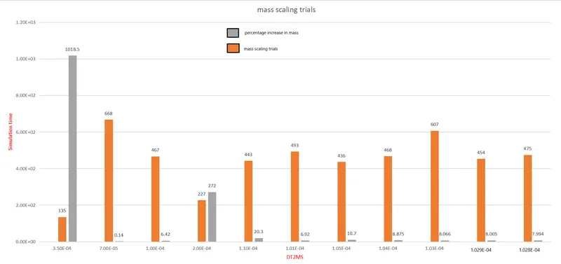
The estimated time required to complete the simulation is around 23 hours or 1380 minutes without mass scaling applied.From the histogram it is clear that the simulation time decreases as the percentage of mass added increases or as the DT2MS value (absolute value) increases. From the graph we can understand that the simulation time is reduced to 475 minutes with eight percent mass scale limit .This also points to us that mass scaling can be used to decrease the simulation time drastically. In our case the simulation time was decreased by about 65.5 %. Eventhough the simulation time can be decreased further at the cost increasing the percentage of mass added it will cause unwanted effects like inertia, which can be a point of concern.

The results obtained after variation of TSSFAC parameter for three DT2MS values is shown below.

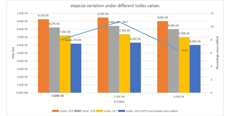
From the above graph it is clear that timestep decreases as TSSFAC parameter is reduced in all the three cases. Also the percentage of mass added is not affected by variation of TSSFAC. This can be useful when we may want to increase the stability without changing the DT2MS value. Since the timestep decreases as we reduce the TSSFAC value the simulation time also goes up but since timestep is reduced stability is increased.

The same problem is run using implicit methord and the time taken to solve the problem is about 62 seconds. Compared to explicit solver the implicit solver solved it very fast as initial timestep(6s) and the following step sizes are very higher than the explicit solver. Implicit solver should only be used when the problems are static or quasi static in nature and also when there is little non linearity. If the problem was very non linear or dynamic then implicit solver may not be able to solve the problem fast and thats where explicit solver shines.