Week - 8 Mass Scaling

OBJECTIVE:

1) To learn about the mass scaling Technique to reduce the computational time for the analysis.

2) The limit for the mass scaling is restricted to 8% and simulation has to be completely stable.

3) Finally, we have to run the same model using an implicit solver with necessary changes and compare implicit and explicit runtime.

INTRODUCTION:-

-> LS-DYNA is an advanced general-purpose multiphysics simulation software package and its origins and core competency lie in highly nonlinear transient dynamic finite element analysis (FEA) using explicit time integration. LS-DYNA is used by the automobile, aerospace, construction and civil engineering, military, manufacturing, and bioengineering industries.

-> Mass-scaling is a term that is used for the process of scaling the element’s mass in explicit simulations to adjust its timestep. The primary motivation is to change (usually increase) the global compute timestep which is limited by the Courant’s stability criteria. Courant Friedrichs Levy's condition for convergence gives a stable time step for explicit analysis. LS-DYNA allows two different types of mass-scaling using the DT2MS parameter from *CONTROL_TIMESTEP with the default set to no mass-scaling. When DT2MS is less than zero, LS-DYNA adds a mass of each element whose timestep(DT) is below required (DT2MS) such that the element’s updated DT is equal to required (DT2MS). When DT2MS is greater than zero, LS-DYNA adds mass to elements whose DT is below required (DT2MS) and “removes” mass from elements whose DT is greater than required (DT2MS). DT2MS>0 is seldom used while DTM2<0 is frequently used for overcoming the smallest computed timestep.

-> Care must be taken when using DT2MS<0 to ensure that the added mass does not have an adverse effect on the simulation accuracy because adding mass can increase the inertia effect in the simulation and that too non physical so It is common practice to limit the percentage of added mass to less than 10% of the overall domain in dynamic simulations but this percentage value is not universal for all the domain in fact it is domain specific so it can get increased or decreased accordingly.

-> Anytime nonphysical mass is added to increase the timestep in a dynamic analysis, results (think of F=ma) are affected. Sometimes this effect is insignificant and in those cases adding nonphysical mass is justifiable.

Timestep:- In FEA, time step is the time required for a shock wave to propogate across the smallest element. The time step is controlled by the acoustic wave propagation through the material. The step size is dependent on a number of factors including the size of the smallest elements. Usually smaller the element size, the smaller will be the time step size selected by the solver when using an explicit scheme. In larger problems, it can lead to an increase in runtime leading to high computation cost.

The above relationship is called the Courant-Friedrichs-Lewy (CFL) condition and determines the stable time step in an element.

Based on the conditions, the time step can be increased to provide faster solution times by artificially increasing the density of the material by using a technique like mass scaling, lowering the modulus, or by increasing the element size of the mesh.

Mass Scaling:- Mass scaling is defined as a technique in FEA where non-physical mass is added in a structure to achieve a larger timestep size in explicit simulation. Mass scaling deals with this issue by adding and subtracting mass according to set criteria in the solver. The concept is simple, Larger Timestep = Lower Solution Time. The manual form of mass scaling is done independently of the automatic mass scaling invoked with DT2MS in *CONTROL_TIMESTEP.

The mass of small or stiff elements is increased to prevent a very small timestep. This means this additional mass must be used very carefully so that the resulting nonphysical inertia effects do not dominate the global solution.

The control timestep card is used for controlling mass scaling in the model. There are two parameters namely DT2MS (time step size for mass scaling) and TSSFAC (time scale factor for mass scaling). DT2MS value specifies the timestep value for which mass scaling needs to be applied. The TSSFAC value further scales the DT2MS value.

DT2MS -> Negative:- Mass is added to only those elements whose timestep would be less than TSSFAC*(DT2MS). This method significantly increases the overall mass of the domain artificially. This method is recommended.

DT2MS -> Positive:- Mass is added or taken away from elements so that there is no significance change in overall mass.

Relational Aspects:- DT2MS is basically the time step below which the mass will be added to elements so as to increase the timestep of that particular element. This increment in the time step happens because artificial mass is added to the nodes of the element, basically the density of the element at that area is increasing, So when density increases the speed of the wave passing through it will reduce. This will in turn increases the timestep. Increasing the timestep will finish the run in less amount of time as iterations will be reduced. But when there is lot of non-linearities involved in the problem, this usage of higher time steps may skip those non linearities and that will lead to inappropriate results.

If stability is a problem with the default TSSFAC of 0.9, we can try 0.8 or 0.7. If we reduce TSSFAC, we can increase |DT2MS| proportionally so that their product, and hence timestep, is unchanged. TSSFAC doesn’t affect the mass scaling percentage.

In this project, the runtime has to be reduced using mass scaling technique by varying the values of DT2MS and TSSFAC with percentage increase of mass within 8% using Explicit and Implicit analysis.

Since DTMS and TSSFAC are the important parameters in the *CONTROL_TIMESTEP card that affects the timestep and the runtime of the simulation, so we will change these values in each iteration to obtain an optimized runtime with a stable solution and to make sure mass scaling doesn’t go beyond 8%.

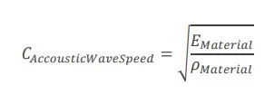
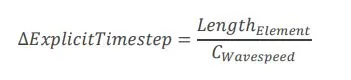
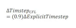
case setup & Execution:

case 1: Run the model without mass scaling

1. The given Keyword file is imported into LS-PrePost, the keyword file consists of all important parameters like mat,sec,boundary conditions, control cards and Data base cards.

2. To understand the process,the *CONTROL_TIMESTEP card is deleted.

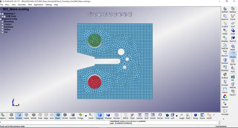
3. The Keyword file is saved in a separate folder and opened in LS-RUN.

Here we can see that the estimated time to complete this simulation is 46 hrs 26 mins which is significantly higher, to reduce this we need to imply mass scaling.

Case 2: With mass scaling

1. *CONTROL_TIMESTEP keyword is added to the model with tssfac=0.9 and DT2MS = -3.500E-05.

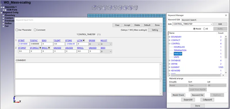
2. The Keyword file is saved in a separate folder and opened in LS-RUN.

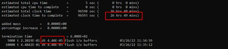
From the above image it can be seen that the time for computation is decreased from 46 hrs 26 mins to 26 hrs 49 mins, the decrease in computation time is not that significant.

But we can see that there is no mass added with given DT2MS of -3.500E-05 with percentage of mass increase in 0%, this can be changed to changing the values of DT2MS and tssfac.

Case 3: Mass scaling with tssfac=0.9 and DT2MS = -3.500E-04

1. *CONTROL_TIMESTEP keyword is added to the model with tssfac=0.9 and DT2MS = -3.500E-04.

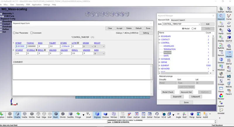
2. The Keyword file is saved in a separate folder and opened in LS-RUN.

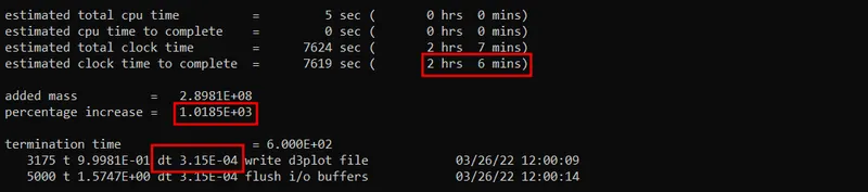
From the above image it can be seen that the time for computation is decreased from 26 hrs 49 mins to 02 hrs 06 mins, there is considerable decrease in computation time.

However we can see that the mass added with given DT2MS of -3.500E-04 with percentage mass increase of 1.0185E+3 is 2.8981E+8.

Since the added mass value exceeding the limit, the energy values will vary considerably and accuracy of the results will be compromised so the given mass needs to be reduced.

Case 4: Mass scaling with tssfac=0.9 and DT2MS = -7.000E-05

1. *CONTROL_TIMESTEP keyword is added to the model with tssfac=0.9 and DT2MS = -7.000E-05.

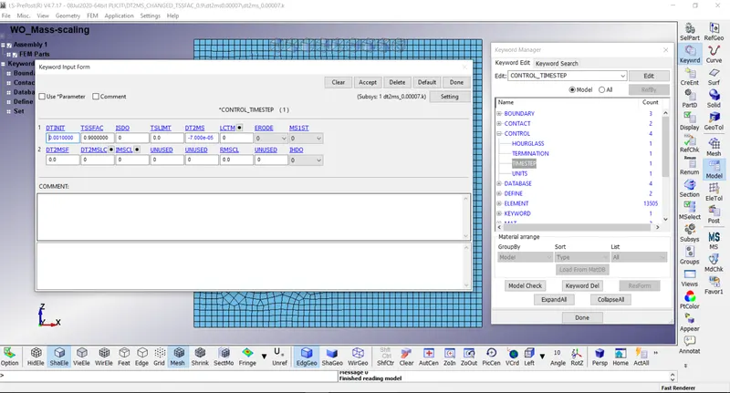
2. The Keyword file is saved in a separate folder and opened in LS-RUN.

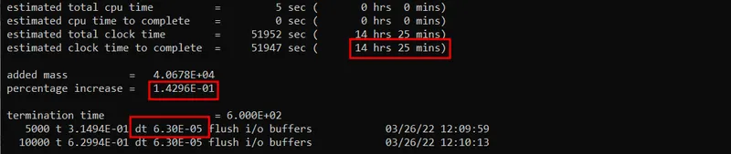
From the above image it can be seen that the computation time is 14 hrs 25 mins which is higher than that of the previous case.

However we can see that the mass added with given DT2MS of -7.000E-05 with percentage mass increase of 1.4296E-01 (i.e., is 0.14%) is 4.0678E+04.

Since it is not the recommended value further mass can be added.

Case 5: Mass scaling with tssfac=0.9 and DT2MS = -9.000E-05

1. *CONTROL_TIMESTEP keyword is added to the model with tssfac=0.9 and DT2MS = -9.000E-05.

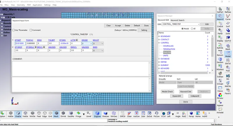
2. The Keyword file is saved in a separate folder and opened in LS-RUN.

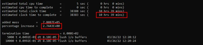
From the above image it can be seen that the computation time is 10 hrs 39 mins which is lesser than that of the previous case.

However we can see that the mass added with given DT2MS of -9.000E-05 with percentage mass increase of 2.7443E+00 (i.e., is 2.7%) is 7.8087E+05.

Since it is not the recommended value further mass can be added.

Case 6: Mass scaling with tssfac=0.9 and DT2MS = -1.000E-04

1. *CONTROL_TIMESTEP keyword is added to the model with tssfac=0.9 and DT2MS = -1.000E-4.

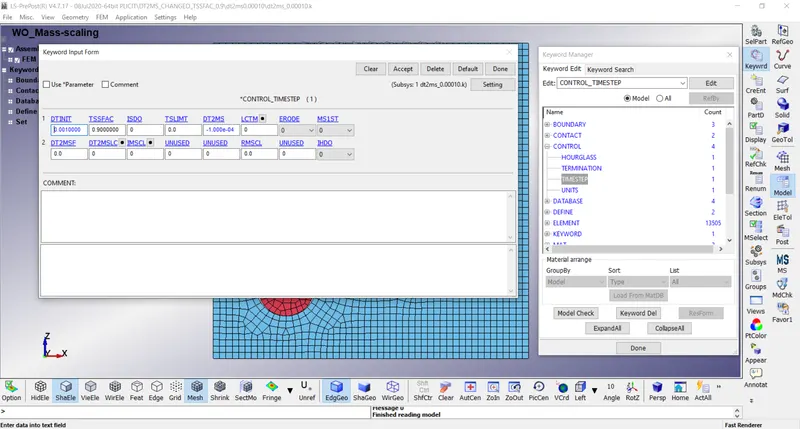
2. The Keyword file is saved in a separate folder and opened in LS-RUN.

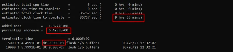
From the above image it can be seen that the computation time is 09 hrs 55 mins which is lesser than that of the previous case.

However we can see that the mass added with given DT2MS of -1.000E-04 with percentage mass increase of 6.4233E+00 (i.e., is 6.4%) is 1.8277E+06.

Since it is not the recommended value further mass can be added.

Case 7: Mass scaling with tssfac=0.9 and DT2MS = -1.100E-04

1. *CONTROL_TIMESTEP keyword is added to the model with tssfac=0.9 and DT2MS = -1.100E-4.

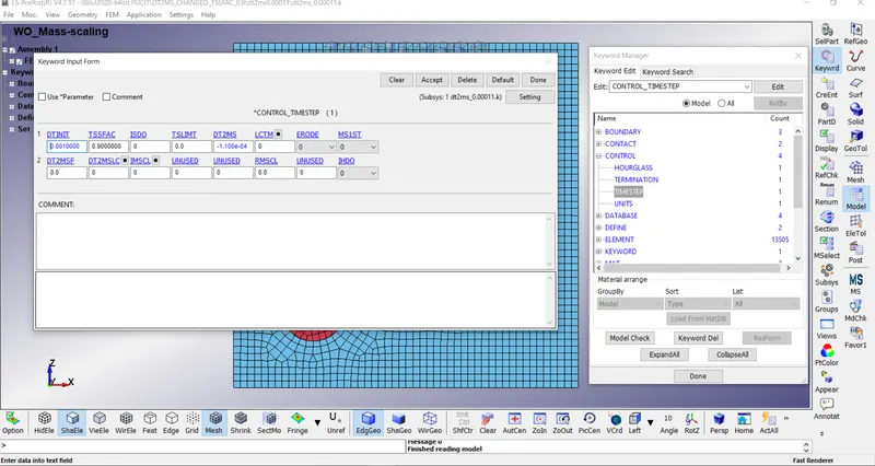
2. The Keyword file is saved in a separate folder and opened in LS-RUN.

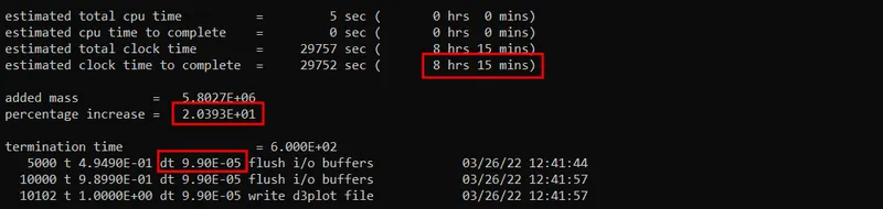
From the above image it can be seen that the computation time is 08 hrs 15 mins which is lesser than that of the previous case.

However we can see that the mass added with given DT2MS of -1.100E-04 with percentage mass increase of 2.0393E+01 (i.e., is 20.4%) is 5.8027E+06.

Since it is not the recommended value further mass can be reduced.

Case 8: Mass scaling with tssfac=0.9 and DT2MS = -1.0100E-04

1. *CONTROL_TIMESTEP keyword is added to the model with tssfac=0.9 and DT2MS = -1.0100E-4.

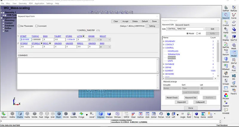
2. The Keyword file is saved in a separate folder and opened in LS-RUN.

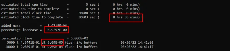
From the above image it can be seen that the computation time is 08 hrs 30 mins which is lesser than that of the previous case.

However we can see that the mass added with given DT2MS of -1.0100E-04 with percentage mass increase of 6.9297E+00 (i.e., is 6.9%) is 1.9718E+06.

Since it is not the recommended value further mass can be added.

Case 9: Mass scaling with tssfac=0.9 and DT2MS = -1.0200E-04

1. *CONTROL_TIMESTEP keyword is added to the model with tssfac=0.9 and DT2MS = -1.0200E-4.

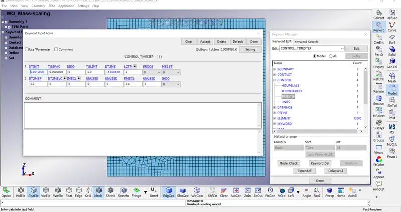
2. The Keyword file is saved in a separate folder and opened in LS-RUN.

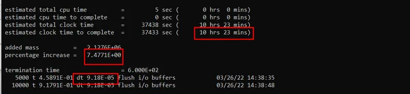
From the above image it can be seen that the computation time is 10 hrs 23 mins which is lesser than that of the previous case.

However we can see that the mass added with given DT2MS of -1.0200E-04 with percentage mass increase of 7.4771E+00 (i.e., is 7.5%) is 2.1276E+06.

Since it is not the recommended value further mass can be added.

Case 10: Mass scaling with tssfac=0.9 and DT2MS = -1.0300E-04

1. *CONTROL_TIMESTEP keyword is added to the model with tssfac=0.9 and DT2MS = -1.0300E-4.

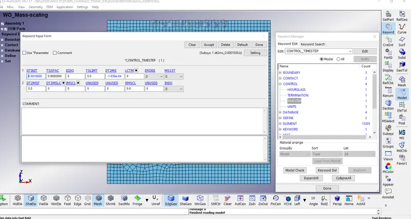
2. The Keyword file is saved in a separate folder and opened in LS-RUN.

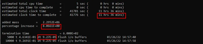
From the above image it can be seen that the computation time is 11 hrs 36 mins which is lesser than that of the previous case.

However we can see that the mass added with given DT2MS of -1.0300E-04 with percentage mass increase of 8.0661E+00 (i.e., is 8.066%) is 2.2952E+06.

Since it is not the recommended value further mass can be reduced.

Case 11: Mass scaling with tssfac=0.9 and DT2MS = -1.0290E-04

1. *CONTROL_TIMESTEP keyword is added to the model with tssfac=0.9 and DT2MS = -1.0290E-4.

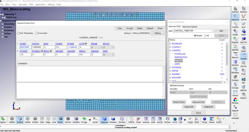
2. The Keyword file is saved in a separate folder and opened in LS-RUN.

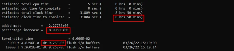
From the above image it can be seen that the computation time is 08 hrs 50 mins which is lesser than that of the previous case.

However we can see that the mass added with given DT2MS of -1.0290E-04 with percentage mass increase of 8.0050E+00 (i.e., is 8.00%) is 2.2778E+06.

In this case the accurate result is achieved with the added mass percentage of 8%.

-> We see that as expected the estimated time (to complete) has reduced and If we notice the mass percentage is 8% which have reached its limit value because more than 8% of the mass is not accepted, So further decreases of DT2MS will only increase and the mass percentage of the system. Therefore from the next case, we vary the TSSFAC (Time Scale Factor) to find whether it has any change in the mass percentage and estimated time.

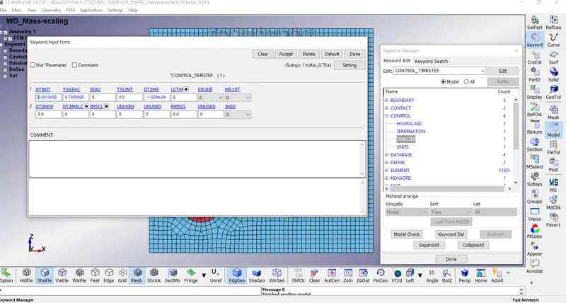
Case 12: Mass scaling with tssfac=0.8 and DT2MS = -1.0290E-04

1. *CONTROL_TIMESTEP keyword is added to the model with tssfac=0.8 and DT2MS = -1.0290E-4.

2. The Keyword file is saved in a separate folder and opened in LS-RUN.

We get the estimated time: 05 hrs 42 mins and the added mass: 8.005%.

Case 13: Mass scaling with tssfac=0.7 and DT2MS = -1.0290E-04

1. *CONTROL_TIMESTEP keyword is added to the model with tssfac=0.7 and DT2MS = -1.0290E-4.

2. The Keyword file is saved in a separate folder and opened in LS-RUN.

We get the estimated time: 14 hrs 05 mins and the added mass: 8.005%.

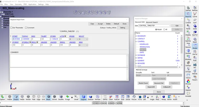
Case 14: Mass scaling with tssfac=0.6 and DT2MS = -1.0290E-04

1. *CONTROL_TIMESTEP keyword is added to the model with tssfac=0.6 and DT2MS = -1.0290E-4.

2. The Keyword file is saved in a separate folder and opened in LS-RUN.

We get the estimated time: 11 hrs 46 mins and the added mass: 8.005%.

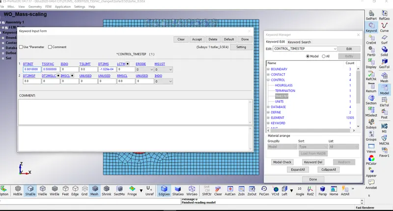
Case 15: Mass scaling with tssfac=0.5 and DT2MS = -1.0290E-04

1. *CONTROL_TIMESTEP keyword is added to the model with tssfac=0.5 and DT2MS = -1.0290E-4.

2. The Keyword file is saved in a separate folder and opened in LS-RUN.

We get the estimated time: 14 hrs 08 mins and the added mass: 8.005%.

-> We see that the time scale factor doesn't change the amount or percentage of mass added as the mass percentage remains the same but the computation time varies inversely according to the Time scale factor.

Implicit Analysis:

Now we will run this same file using an implicit solver. Additional control cards are used to run this simulation in an implicit solver.

• Control cards

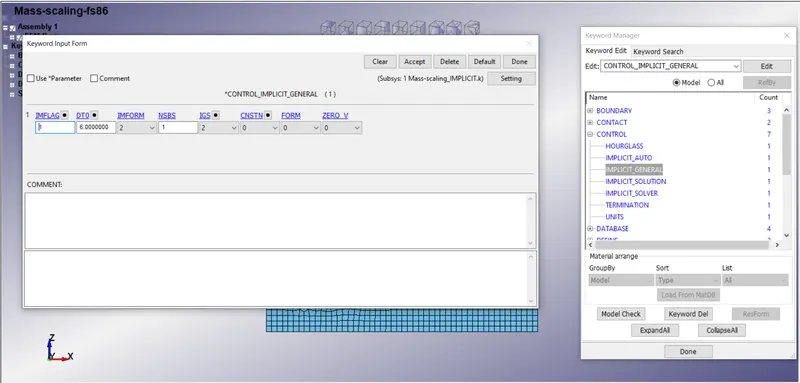
1.*CONTROL_IMPLICIT_GENERAL

Activate implicit analysis and define associated control parameters. This keyword is mandatory to define for all implicit analyses.

• IMFLAG: Implicit/Explicit analysis type flag: 1- implicit analysis.
• DT0: Initial time step size for implicit analysis (Termination time/100).

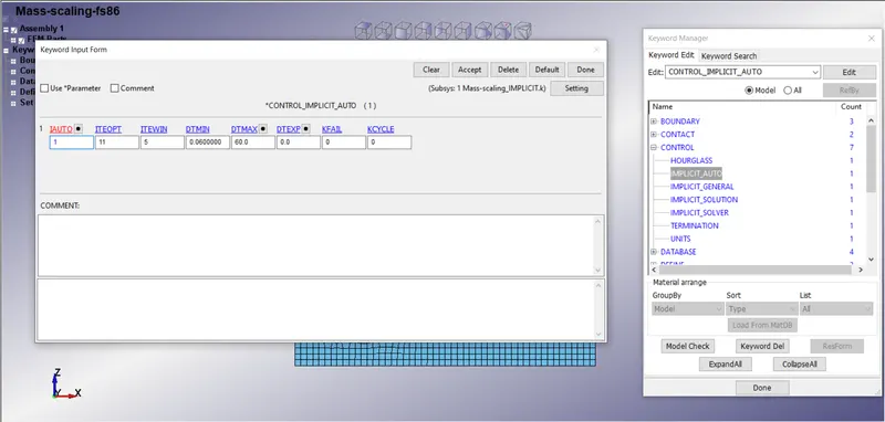
2.*CONTROL_IMPLICIT_AUTO:

• IAUTO: 1 - automatically adjust the time step size.
• ITEOPT: Optimum equilibrium iteration count per time step.
• ITEWIN: Allowable iteration window. If the iteration count is within the range of (ITEOPT+ITEWIN) - (ITEOPT-ITEWIN), the step size will not be adjusted.
• DTMIN: Minimum allowable time step size (DT/100).
• DTMAX: Maximum allowable time step size (default = DT*10).

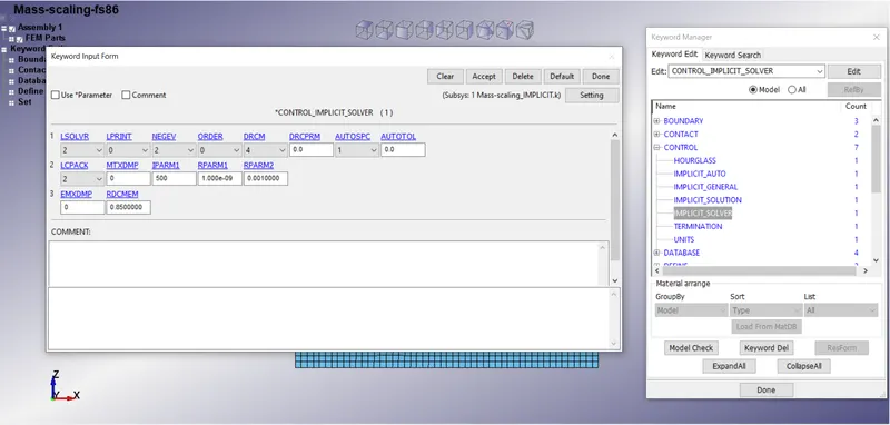
3.*CONTROL_IMPLICIT_SOLVER

The linear equation solver performs the CPU-intensive stiffness matrix inversion.

• LSOLVR: Parallel multi-frontal sparse solver (default).

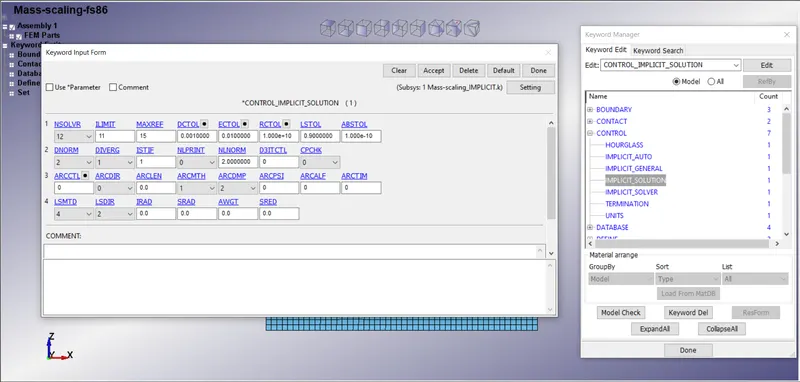
4.*CONTROL_IMPLICIT_SOLUTION

Use of these cards to specify whether a linear or nonlinear solution is desired.

• NSOLVER: Solution method for implicit analysis: 12 For Non-linear problem.
• ILIMIT: Iteration limit between automatic stiffness reformations: 11
• MAXREF: Stiffness reformation limit per time step: 15
• DCTOL: Displacement relative convergence tolerance: 0.001
• DNORM: Displacement norm for convergence test: 2 (Increment as a function of total displacement).

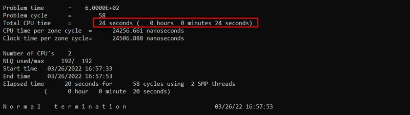
The Keyword file is saved in a separate folder and opened in LS-RUN.

RESULTS:-

Histogram -

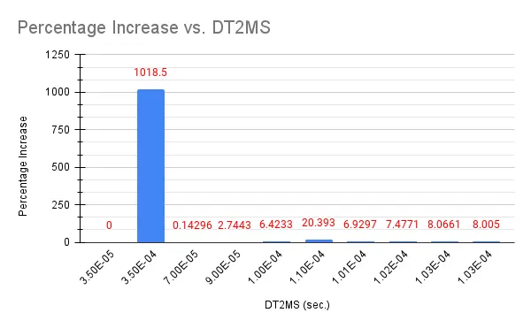
1. % Increase in Mass vs. DT2MS (Keeping TSSFAC = 0.9)

The Percentage Increase vs DT2MS plot shows that when we add mass to the model using the DT2MS as the value of it increases, the estimated simulation time decreases infact % mass increases by a whopping 1018% of the total domain mass when DT2MS is increased by an order of 10, so we can go with a % increase in mass of 8.005%, acceptable for this case.

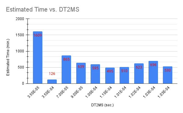
2. Estimated Time vs. DT2MS (Keeping TSSFAC = 0.9)

The DT2MS vs Estimated Time shows that when we add mass to the model using the DT2MS as the value of it increases, the estimated simulation time decreases.

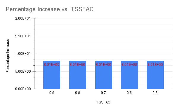
3. % Increase in Mass vs. TSSFAC (Keeping DT2MS = 0.0001029)

% Increse in mass vs. TSSFAC plot shows that while keeping DT2MS fixed, increasing TSSFAC doesn't affect the % increase in mass at all.

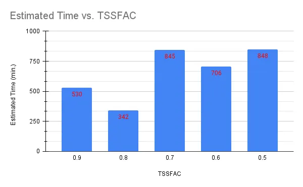
4. Estimated Time vs. TSSFAC (Keeping DT2MS = 0.0001029)

The Estimated TSSFAC vs Time shows that when DT2MS value is fixed and changed the TSSFAC values which don't add mass to the model as seen from the above cases the mass percentage remains the same because of which the estimated simulation time increases with decrement in TSSFAC value.

CONCLUSIONS:-

Comparison between explicit and implicit runtime -

As it is clear, the implicit scheme was very fast. It can be attributed to the fact that in the implicit scheme the concept of time is not exactly time. It can be thought of as load steps. Also, there is not any limitation on timestep size which enabled us to use high timestep size for a single time step.

As we know, Explicit FEM is used to calculate the state of a given system at a different time from the current time. In contrast, an implicit analysis finds a solution by solving an equation that includes both the current and later states of the given system. In Implicit analysis, each time step has to converge, but we can set pretty long time steps and it is based on iterations. Explicit on the other hand doesn’t have to converge each time step, but for the solution to be accurate time steps must be small. Though the running time for implicit analysis is shorter than the explicit analysis method because the timestep is defined larger in implicit analysis compare to explicit without compromising with the accuracy of the solution because of unconditionally stable solutions.

1) We have learned about the mass scaling Technique to reduce the computational time for the analysis.

2) We have also brought mass scaling percentage to 8% by varying the DT2MS values and then we have also found that mass addition doesn't depend on the TSSFAC (Time Step Factor) in the model.

3) After, that we have run the analysis using implicit control cards which gives us the result that the implicit analysis is based on iterations and doesn't depend on mass scaling, also implicit analysis gives fast results with convergence.

4) Finally, we also compared explicit and implicit analysis, also we have plotted the histogram for DT2MS vs Estimated Time and TSSFAC vs Estimated Time by interchanging quantities.