Week 8: Literature review - RANS derivation and analysis

Objective: -

1. Discuss Reynold’s stress. Derive an expression for Reynold’s stress by applying Reynold’s decomposition to the NS equations.
2. Discuss Turbulent viscosity and how is it different from molecular viscosity.

Theory: -

Turbulence: -

In fluid dynamics, turbulence or turbulent flow is fluid motion characterized by chaotic changes in pressure and flow velocity. It is in contrast to a laminar flow, which occurs when a fluid flows in parallel layers, with no disruption between those layers.Turbulence is caused by excessive kinetic energy in parts of a fluid flow, which overcomes the damping effect of the fluid's viscosity. This increases the energy needed to pump fluid through a pipe.

The onset of turbulence can be predicted by the dimensionless Reynolds number, the ratio of kinetic energy to viscous damping in a fluid flow.

a. For Internal Flows – Re > 4000 b. For external Flows – Re > 3,00,000

Navier-Stokes equations –

These are certain partial differential equations which describe the motion of viscous fluid substances. They mathematically express conservation of momentum and conservation of mass for Newtonian fluids. They are sometimes accompanied by an equation of state relating pressure, temperature and density.

Together with continuity equation they are solved to describe the fluid flow phenomena and are called Governing Equations of fluid flow. The equations at boundary layer are –

Continuity Equation - Conservation of Mass

`ρ[(∂u)/(∂x)+(∂v)/(∂y)]=0`

Momentum Equation - Conservation of Momentum

`ρ[(∂u)/(∂t)+u*(∂u)/(∂x)+v*(∂u)/(∂y)]=-(∂P)/(∂x)+μ((∂^2 u)/(∂x^2 )+(∂^2 u)/(∂y^2 ))`

Energy/Transport Equation - Conservation of Energy

`ρC_P [(∂T)/(∂t)+u*(∂T)/(∂x)+v*(∂T)/(∂y)]=K*(∂^2 T)/(∂x^2 )+μ((∂u)/(∂y))^2`

Turbulence Modelling-

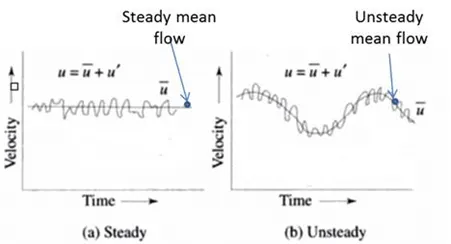
Implementation of the turbulence model into the numerical scheme is substantial and makes a big difference to the simulation results. The main purpose of turbulence modelling is to prompt equations to anticipate the time-averaged velocity, pressure, and temperature fields, without calculating the complete turbulent flow pattern

`u(x,y,z,t)=ubrace(baru(x,y,z))+ubrace(u'(x,y,z,t))`

Time Averaged Fluctuating

The three main turbulence model can be summarised as follow:

1. Direct Numerical Simulation (DNS): Direct implementation of fluctuated values into the Navier-Stokes equation without any turbulence model.
2. Large Eddy Simulation (LES): An average turbulence model between DNS and RANS in which filtered Navier-Stokes equations are used for large-scale eddies. An appropriate model is preferred to solve small-scale eddies.
3. Reynolds-Averaged Navier-Stokes equations (RANS): A mathematical model based on average values of variables for both steady-state and dynamic flows (unsteady for URANS). The numerical simulation is driven by a turbulence model which is arbitrarily selected to find out the effect of turbulence fluctuation on the mean fluid flow.

In RANS model the properties are addition two components one averaged while other fluctuating as velocity as function of time shown below

`bar u` is Averaged quantity and u’ is fluctuating quantity and u is instantaneous quantity. This breakdown of variable is called Reynolds Decomposition.

Applying Reynolds decomposition on NS equations

Continuity equation:

`ρ[(∂u)/(∂x)+(∂v)/(∂y)]=0`

putting u = `bar u` +u’ and v= `bar v` + v’ , we get

`[(∂(bar u + u'))/(∂x)+(∂(bar v + v'))/(∂y)]= 0`

`(∂bar u)/(∂x) + (∂u')/(∂x) + (∂bar v)/(∂y) + (∂v')/(∂y) = 0`

integrating over time step t, we get

`(1/t)int_0^t(∂bar u)/(∂x) dt + (1/t)int_0^t(∂u')/(∂x)dt + (1/t)int_0^t(∂bar v)/(∂y)dt + (1/t)int_0^t(∂v')/(∂y)dt = 0`

since the time average of fluctuating quantity is 0 and time average of average gives constant value hence after elemination, we get

`(∂bar u)/(∂x) *(1/t)int_0^tdt + (∂bar v)/(∂x) *(1/t)int_0^tdt = 0`

`(∂bar u)/(∂x) + (∂bar v)/(∂x) = 0`

Momentum equation:

`ρ[(∂u)/(∂t)+u*(∂u)/(∂x)+v*(∂u)/(∂y)]=-(∂P)/(∂x)+μ((∂^2 u)/(∂x^2 )+(∂^2 u)/(∂y^2 ))`

adding continuity eqution to both side and rearranging, we get

`(∂u)/(∂t)+u(∂u)/(∂x)+v(∂u)/(∂y) + u((∂u)/(∂x)+(∂v)/(∂y))=-1/ρ(∂P)/(∂x)+ν((∂^2 u)/(∂x^2 )+(∂^2 u)/(∂y^2 ))`

As `2u(du)/dx = (du^2)/dx` and `u(dv)/dy +v(du)/dy = (duv)/dy`, we get

`(∂u)/(∂t)+2u(∂u)/(∂x)+(∂uv)/(∂y) =-1/ρ(∂P)/(∂x)+ν((∂^2 u)/(∂x^2 )+(∂^2 u)/(∂y^2 ))`

putting u = `bar u`+u’ , v= `bar v`+ v’ and P = `barP + P'`, we get

`(∂(baru+u'))/(∂t)+2(baru+u')(∂(baru+u'))/(∂x)+(∂(baru+u')(barv+v'))/(∂y) =-1/ρ(∂(barP+P'))/(∂x)+ν((∂^2(baru+u'))/(∂x^2 )+(∂^2(baru+u'))/(∂y^2 ))`

integrating over time step t and eliminating the time integral u', v' and P' as they are fluctuating and are equal to 0, we get

`1/t int_0^t (dbaru)/dt dt +1/t int_0^t (dbaru^2)/dx dt +1/t int_0^t (du'^2)/dx dt + 1/t int_0^t (duv)/dy dt +1/t int_0^t (du'v')/dy dt = 1/t int_0^t 1/t (dbarP)/dx dt + 1/t int_0^t ν (d^2 baru)/(dx^2) dt 1/t int_0^t ν (d^2 baru)/(dy^2) dt`

On integrating and rearranging the terms, equation reduces to

`(∂u)/(∂t)+(∂baru^2)/(∂x)+(∂baru barv)/(∂y) =-1/ρ(∂barP)/(∂x)+ν((∂^2baru)/(∂x^2 )+(∂^2baru)/(∂y^2))- 1/t int_0^t (du'v')/(dy) dt - 1/t int_0^t (du'^2)/(dy) dt`

As `int_0^t (du')/dx dt = 0` But `int_0^t (du'^2)/dx dt != 0`

but since the gradient along x axis is very small and its square make it comparibaly very small to y gradients, Hence this term is negected and integration term re replaced with average terms.

`(∂u)/(∂t)+(∂baru^2)/(∂x)+(∂baru barv)/(∂y) =-1/ρ(∂barP)/(∂x)+ν((∂^2baru)/(∂x^2 )+(∂^2baru)/(∂y^2))- color(red)((dbar(u'v'))/(dy) - (dbar(u'^2))/(dy))`

Here the stress term is highlighted in red which is written in the form -

`ubrace(mu(dbar(u'v'))/(dy))_( "Reynolds stress gradient") - ubrace(rho(dbar(u'^2))/(dy))_("shear stress gradient")` `=> d[ mu (du)/(dy) - rho bar(u'v')]/dy`

`"Total Stress" =ubrace(mu (du)/(dy))_("Laminar")- ubrace(rho bar(u'v'))_("Turbulent")`

Reynold’s Stress –

It is the component of the total stress tensor in a fluid obtained from the averaging operation over the Navier–Stokes equations to account for turbulent fluctuations in fluid momentum.

`tau = rho bar(u'v')`

Energy equation:

`ρC_P [(∂T)/(∂t)+u*(∂T)/(∂x)+v*(∂T)/(∂y)]=K*(∂^2 T)/(∂x^2 )+μ((∂u)/(∂y))^2`

putting u = `bar u`+u’ , v= `bar v`+ v’ and T = `barT + T'`, we get

`ρC_P [(∂(barT+T'))/(∂t)+(baru+u')*(∂(barT+T'))/(∂x)+(barv+v')*(∂(barT+T'))/(∂y)]=K*(∂^2(barT+T'))/(∂x^2 )+μ((∂(baru+u'))/(∂y))^2`

On expanding , Integrating and eleminating , we get

`ρC_P [(∂(barT))/(∂t)+(baru)(∂(barT))/(∂x)+1/t int_0^tu'(dT')/(dx) dt + barv (dbarT)/dy +1/t int_0^tv'(dT')/(dy) dt] =K*(∂^2(barT))/(∂x^2)+μ[((∂(baru))/(∂y))^2+ 1/t int_0^t ((du')/(dy))^2 dt ]`

Here the integeral terms are the one which are in addition to the equation for mean values. Adding `T'(du')/(dx) + T'(dv')/(dy)` as it's value is 0, we get

`ρC_P [(∂(barT))/(∂t)+baru(∂(barT))/(∂x)+ barv (dbarT)/dy + ubrace((d(bar(u'T')))/(dx) + (d(bar(v'T')))/(dy))_("Turbulent flux") ]=K*ubrace((∂^2(barT))/(∂x^2))_("Molecular flux")+ubrace(μ((∂(baru))/(∂y))^2)_("Viscous stress Dissipation")+ubrace(μ((∂(baru'))/(∂y))^2)_("turbulent stress issipation")`

`"Total flux" (q) = ubrace(-k (dbarT)/dx)_("Molecular Flux") - ubrace( rho C_p bar(u'T') )_("Turbulent flux")`

Turbuent Viscosity: -

It is also called as eddy viscosity. In the study of turbulence in fluids, a common practical strategy is to ignore the small-scale vortices (or eddies) in the motion and to calculate a large-scale motion with an effective viscosity, called the "eddy viscosity", which characterizes the transport and dissipation of energy in the smaller-scale flow (see large eddy simulation). In contrast to the viscosity of the fluid itself, which must be positive by the second law of thermodynamics, the eddy viscosity can be negative.

Molecular Viscosity: -

It is the transport of mass motion momentum solely by the random motions of individual molecules not moving together in coherent groups. Molecular viscosity is analogous in laminar flow to eddy viscosity in a turbulent flow.