Understanding RANS equation derivation and analysis
The Navier stokes equations are so powerful that they can be applied to the boundary layer as well. For a boundary layer, the NS equations are as follows.
Continuity equation: -
`frac{partial u}{partial x}+frac{partial v}{partial y}=0`
Momentum equation: - (along X)
`rho(frac{partial u}{partial t}+ufrac{partial u}{partial x}+vfrac{partial u}{partial y})=-frac{dP}{dx}+frac{mupartial^2u}{partial y^2}`
Energy equation: - (2D)
`rho_C(frac{partial T}{partial t}+ufrac{partial T}{partial x}+vfrac{partial T}{partial y})=kfrac{partial^2T}{partial x^2}+mu(frac{partial u}{partial y})^2`
In the above equations, it is obvious that some terms are missing, this is because those terms can be neglected in a boundary layer when their magnitude is considered.
The above 3 equations can be solved to obtain all effects of the flow including turbulence. This process is called Direct Numerical Simulation. But at the boundary layer, over the turbulent region, the velocity keeps changing over a small period. This time is called the turbulent time scale which is very small. Also, the velocity change occurs over a very small distance. If we use DNS for these small distances with a huge number of cells, we can capture the turbulence, but the simulation is going to take forever to finish. So, we use turbulence models.
We take these governing equations and integrate them over a time step that is much larger than the turbulent time scale. This process is called averaging. We apply the Reynolds decomposition
Reynold’s decomposition
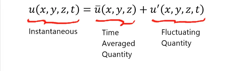
In Reynolds decomposition, we divide the flow variables into a sum of a mean variable and a fluctuating variable.
`bar{u}(x,y)=frac{1}{t_{"int"}}int_{0}^{t_{"int"}}u(x,y,t)dt`
`t_{"int"}`= integration time
`bar{v}(x,y)=frac{1}{t_{"int"}}int_{0}^{t_{"int"}}v(x,y,t)dt`
Now,`u(x,y,z,t)=bar{u}(x,y,z)+u^'(x,y,z,t)`
Applying integration over tint to the above equation we get
`frac{1}{t_{"int"}}int_{0}^{t_{"int"}}u(x,y,z,t)dt=frac{1}{t_{"int"}}int_{0}^{t_{"int"}}{bar{u}(x,y,z)dt}+frac{1}{t_{"int"}}int_{0}^{t_{"int"}}{u^'(x,y,z,t)dt}`
In the above equation the value of `frac{1}{t_{"int"}}int_{0}^{t_{"int"}}{bar{u}(x,y,z)dt} = frac{1}{t_{"int"}}int_{0}^{t_{"int"}}u(x,y,z,t)dt`
Because if the average of is and if we take the average of we get the same quantity again. Just like the average of 1,2,3,4,5 is 7.5 and if take the average of 7.5,7.5,7.5,7.5,7.5 is 7.5 again. So, we get
`frac{1}{t_{"int"}}int_{0}^{t_{"int"}}{u^'(x,y,z,t)dt} = 0`
It means whenever we apply the time-averaged integration on a fluctuating component it is = 0.
This can be applied to all other components like T, P, etc.
Applying the above procedure for NS equations we get
Continuity equation
`frac{partial u}{partial x}+frac{partial v}{partial y}=0`
`frac{partial}{partial x}(bar{u}+u^')+frac{partial}{partial y}(bar{v}+v^')=0`
Integrating the above equation over tint
`frac{1}{t_{"int"}}intfrac{partial}{partial x}(bar{u}+u^prime)dt+frac{1}{t_{"int"}}intfrac{partial}{partial y}(bar{v}+v^')dt=0`
If we expand the above integration
`frac{1}{t_{"int"}}intfrac{partialbar{u}}{partial x}dt+frac{1}{t_{"int"}}intfrac{partial u^'}{partial x}dt+frac{1}{t_{"int"}}intfrac{partialbar{v}}{partial y}dt+frac{1}{t_{"int"}}intfrac{partial v^'}{partial y}dt=0`
We know that the time-averaged integral of fluctuating terms is equal to 0 therefore `frac{1}{t_{"int"}}intfrac{partial u^'}{partial x}dt=0;frac{1}{t_{"int"}}intfrac{partial v^'}{partial y}dt=0`
We are left with `frac{1}{t_{"int"}}intfrac{partialbar{u}}{partial x}dt+frac{1}{t_{"int"}}intfrac{partialbar{v}}{partial y}dt=0` here the mean terms are not a function of time hence
`frac{partialbar{u}}{partial x}+frac{partialbar{v}}{partial y}=0`
In other words, the above equation represents that the time-averaged velocity components satisfy the continuum equation.
Momentum equation
`rho(frac{partial u}{partial t}+ufrac{partial u}{partial x}+vfrac{partial u}{partial y})=-frac{dP}{dx}+mufrac{partial^2u}{partial y^2}`
Taking density to RHS we get
`frac{partial u}{partial t}+ufrac{partial u}{partial x}+vfrac{partial u}{partial y}=frac{1}{rho}frac{-dP}{dx}+frac{mu}{rho}frac{partial^2u}{partial y^2}`
We know that `frac{mu}{rho} = vartheta` which is the kinematic viscosity
`frac{partial u}{partial t}+ufrac{partial u}{partial x}+vfrac{partial u}{partial y}=frac{-dP}{rhodx}+varthetafrac{partial^2u}{partial y^2}`
On the LHS we add the continuity expression multiplied with u to convert the above equation into a more suitable form.
Adding the continuity expression will not make a difference since the continuity expression equals = 0
`frac{partial u}{partial t}+ufrac{partial u}{partial x}+vfrac{partial u}{partial y}+u(frac{partial u}{partial x}+frac{partial v}{partial y})=-frac{dP}{rhodx}+varthetafrac{partial^2u}{partial y^2}`
`frac{partial u}{partial t}+2ufrac{partial u}{partial x}+vfrac{partial u}{partial y}+ufrac{partial v}{partial y}=-frac{dP}{rhodx}+varthetafrac{partial^2u}{partial y^2}`
Using the product rule, we can simplify the above equation as follows
`frac{partial u}{partial t}+2ufrac{partial u}{partial x}+frac{partial}{partial y}(uv)=-frac{1}{rho}frac{dP}{dx}+varthetafrac{partial^2u}{partial y^2}`
We know that `frac{partial}{partial x}(u^2)=2ucdotfrac{partial u}{partial x}`
`frac{partial u}{partial t}+frac{partial}{partial x}(u^2)+frac{partial}{partial y}(uv)=-frac{1}{rho}frac{dP}{dx}+varthetafrac{partial^2u}{partial y^2}`
Applying the time integral we get
`frac{1}{t_{"int"}}int_{0}^{t_{"int"}}{frac{partial}{partial t}(bar{u}+u^prime)dt}+ frac{1}{t_{"int"}}int_{0}^{t_{"int"}}{frac{partial}{partial x}(bar{u}+u^prime)^2dt} + frac{1}{t_{"int"}}int_{0}^{t_{"int"}}(frac{partial}{partial y}(bar{u}+u^')(bar{v}+v^')dt`
=
`frac{1}{t_{"int"}}int_{0}^{t_{"int"}}(-frac{1}{rho}(frac{d(bar{P}+P^')}{dx})dt) + frac{1}{t_{"int"}}int_{0}^{t_{"int"}}{varthetafrac{partial^2}{partial y^2}(bar{u}+u^')dt}`
We expand the above equation
`frac{1}{t_{"int"}}int_{0}^{t_{"int"}}{frac{partialbar{u}}{partial t}dt} + frac{1}{t_{"int"}}int_{0}^{t_{"int"}}{frac{partial u^'}{partial t}dt} + frac{1}{t_{"int"}}int_{0}^{t_{"int"}}{frac{partialbar{u^2}}{partial x}dt} + frac{1}{t_{"int"}}int_{0}^{t_{"int"}}{frac{partial {uprime^2}}{partial x}dt} + frac{1}{t_{"int"}}int_{0}^{t_{"int"}}{frac{partial}{partial x}(2.bar{u}cdot u^')dt} + frac{1}{t_{"int"}}int_{0}^{t_{"int"}}{frac{partial}{partial y}(bar{u}cdotbar{v})dt} + frac{1}{t_{"int"}}int_{0}^{t_{"int"}}{frac{partial}{partial y}(bar{u}cdot v^')dt} + frac{1}{t_{"int"}}int_{0}^{t_{"int"}}{frac{partial}{partial y}(u^1cdotbar{v})dt }+ frac{1}{t_{"int"}}int_{0}^{t_{"int"}}{frac{partial}{partial y}(u^primecdot v^')dt}`
`= frac{1}{t_{"int"}}int_{0}^{t_{"int"}}{-frac{1}{rho}frac{partialbar{P}}{partial x}dt}-frac{1}{t_{"int"}}int_{0}^{t_{"int"}}{frac{1}{rho}frac{partial P^prime}{partial x}dt} + frac{1}{t_{"int"}}int_{0}^{t_{"int"}}{varthetafrac{partial^2bar{u}}{partial y^2}dt}+frac{1}{t_{"int"}}int_{0}^{t_{"int"}}{varthetafrac{partial^2u^'}{partial y^2}dt}`
Removing the integrals of fluctuating variables from the above equation we get
`frac{1}{t_{"int"}}int_{0}^{t_{"int"}}{frac{partialbar{u}}{partial t}dt} + frac{1}{t_{"int"}}int_{0}^{t_{"int"}}{frac{partialbar{u}}{partial x}dt} + frac{1}{t_{"int"}}int_{0}^{t_{"int"}}{frac{partial u^{'^2}}{partial x}dt} + frac{1}{t_{"int"}}int_{0}^{t_{"int"}}{frac{partial}{partial y}(bar{u}cdotbar{v})dt} + frac{1}{t_{"int"}}int_{0}^{t_{"int"}}{frac{partial}{partial y}(u^primecdot v^')dt} = frac{1}{t_{"int"}}int_{0}^{t_{"int"}}{-frac{1}{rho}frac{partialbar{p}}{partial x}dt}+ frac{1}{t_{"int"}}int_{0}^{t_{"int"}}{varthetafrac{partial^2bar{u}}{partial y^2}dt}`
It implies
`frac{partialbar{u}}{partial t} + frac{partialbar{u}}{partial x} + frac{partial}{partial y}(bar{u}cdotbar{v}) = -frac{1}{rho}frac{partialbar{P}}{partial x} + varthetafrac{partial^2bar{u}}{partial y^2} - frac{1}{t_{"int"}}int_{0}^{t_{"int"}}{frac{partial}{partial y}(u^primecdot v^')dt} - frac{1}{t_{"int"}}int_{0}^{t_{"int"}}{frac{partial u^{'^2}}{partial x}dt}`
Except for the last two terms on RHS, all other terms were present in the NS equations except that they were not averaged.
At the boundary layer there will be a co-relation between u and v and the gradients in the y-axis are much stronger and larger than gradients in x hence we ignore the terms that square the gradients in x.
Hence the term `- frac{1}{t_{"int"}}int_{0}^{t_{"int"}}{frac{partial u^{'^2}}{partial x}dt}` is neglected and we get the following equation.
`frac{partialbar{u}}{partial t} + frac{partialbar{u}}{partial x} + frac{partial}{partial y}(bar{u}cdotbar{v}) = -frac{1}{rho}frac{partialbar{P}}{partial x} + varthetafrac{partial^2bar{u}}{partial y^2} - frac{1}{t_{"int"}}int_{0}^{t_{"int"}}{frac{partial}{partial y}(u^primecdot v^')dt}`
This equation is called the Reynolds Averaged Navier Stokes equation.
In the above equation, we have the inertial forces on the LHS and on the RHS we have the pressure term, and we have two other terms which are the shear stress terms
In the shear stresses, we have viscous stress which is `varthetafrac{partial^2bar{u}}{partial y^2}`
And we have another stress called the Reynolds stress which is `frac{1}{t_{"int"}}int_{0}^{t_{"int"}}{frac{partial}{partial y}(u^primecdot v^')dt}`
Turbulence modeling of a problem depends upon getting this term correctly.
This means that the momentum of the fluid is diffused by the molecular viscosity and diffusion because of turbulence.
The unknown in the RANS equation is the time integral and we use turbulence modeling to capture it.
In the boundary layer, we know that there are three layers viscous sublayer, the buffer layer, and the turbulent layer.
If we are dealing with viscous sub-layer. The flow will be laminar. In this case, the inertial terms are dominated by the viscous terms and hence inertial terms are neglected. Assuming that there is no pressure drop, we can neglect the pressure terms as well.
Therefore, in the RANS equation the LHS = 0, and in the RHS we have the pressure term zero and we are left with.
`varthetafrac{partial^2bar{u}}{partial y^2} - frac{1}{t_{"int"}}int_{0}^{t_{"int"}}{frac{partial}{partial y}(u^primecdot v^')dt} = 0`
We can rearrange the above equation as
`frac{1}{rho}frac{partial}{partial y}[mufrac{partialbar{u}}{partial y}-frac{rho}{t_{"int"}}int_{0}^{t_{"int"}}u^'v^'dt]=0`
If the differential of a particular term is equal to 0 then that term is a constant. Which means
`mufrac{partialbar{u}}{partial y}-frac{rho}{t_{"int"}}int_{0}^{t_{"int"}}u^'v^'dt` = shear stress = constant
With the same assumptions as above let us assume that we're dealing with the buffer layer then the turbulent stress dominates the viscous stress. Hence, we get
`tau_{s = }-frac{rho}{t_{"int"}}int_{0}^{t_{"int"}}u^'v^'dt`
This means for a buffer layer and above, the shear stress in the flow is the Reynolds stress and upon integrating it we get.
`tau_{s = }- rho u^'v^'`
Turbulent Viscosity:
The turbulent viscosity is a quantity formulated to predict the turbulent flow characteristics. This term is added to molecular viscosity in momentum and energy equations, and this adds to the diffusion mechanism
If we consider a simple shear flow, the fluid element is sheared by both mean flow and eddy/turbulence.
`tau = mu frac{partial u}{partial y}`
The shear stress from the eddies/ turbulence is given by the Reynolds stress which is`tau = - rho uprimevprime`
we assume that the turbulent fluctuations in this fluid flow are analogous to the Brownian motion of gas particles. The turbulent motion isn't random, it is made up of eddies. The fluctuations are all correlated.
In a sheared flow, the lower particles are accelerated by the faster-moving fluid above them. Due to this, there is a net transport of momentum to the lower particles (downwards, In general, the momentum is transported in the direction of the velocity gradient.)
If the velocity in the top layer and if the bottom layer is slower than the top increases the shear stress will increase as well. Hence we can assume that the Reynolds stress is proportional to the velocity gradient. If the turbulence is stronger then the greater the momentum diffusion from top to bottom.
therefore we can come up with the following expression,
`-rhouprimevprime = mu_t frac{partial u}{partial y}`
`mu_t = frac{-rhouprimevprime}{frac{partialu}{partialy}}`
This is also called the Boussinesq approximation or Boussinesq Hypothesis or eddy viscosity model.
Where `mu_t` is artificial and can control the strength of diffusion.
Therefore, for 1D we have `-rhouprimevprime = mu_t frac{partial u}{partial y}`
Similarly in the y-direction, we have `-rhouprimevprime = mu_t frac{partial v}{partial x}`
So upon adding the above two equations, we get
`-rhouprimevprime = mu_t/2 {frac{partial u}{partialy}+frac{partial v}{partial x}}`
The combined equations for normal stress and shear stress are given by
`-rho uprime u prime = mu_t {(nablau)+(nablau)^T-2/3(nablau)I}-2/3rhokI`
where k is the kinetic energy, 'I' is the identity matrix
Another form to represent the normal and shear stress in the fluid is given by
`S_{ij} = 1/2{frac{del U_i}{delx_j}+frac{delU_j}{delx_i}-1/3frac{delU_k}{x_k}delta_{ij}}`
`-rhou_i^'u_j^' = 2mu_t(s_{ij}-1/3frac{delu_k}{delx_k}S_{ij})-2/3rhokS_{ij}`
`-rhou_j^'u_j^'= 2mu_tS_{ij}^* -2/3rhokdelta_{ij}`
How is it calculated?
Based on the turbulence model (for example `k-epsilon`)
`mu_t = rho C_mufrac{k^2}{epsilon}`
we solve an equation for k and `epsilon`from this we calculate `mu_t`
from `mu_t`we find out the Reynolds stresses.
We can also find the Dynamic turbulent viscosity `mu_t=frac{vartheta_t}{rho}`
However, for flows that have sharp turns / strong curvature / impinging jets / axial strain / sudden change in flow directions these methods to calculate the turbulent viscosity may not work.
For those kind, we should use other models such as Reynolds stress, Non-linear Eddy viscosity models or LES