Week 7 State of charge estimation

1. 

Following the steps from the Simulation of the BMS Model in Simulink in FAQ, the BMS Closed Loop Harness Board is shown below.

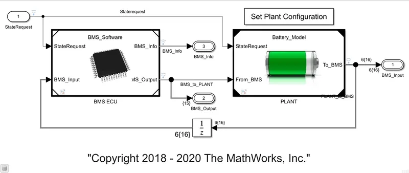
The BMS model comprises a BMS ECU (electrical control unit) and a plant. The control unit is connected to a block representing the battery pack and associated circuitry and peripherals with various monitoring and control algorithms. This model contains two versions of the battery pack: a small one with just six cells series and a larger 16-module pack, each module containing a 6-cell series string. The architecture is 6S-1P and 96S-1P packs, respectively.

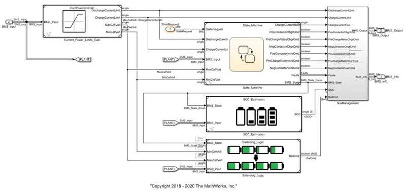
When We click on the BMS ECU, its subsystem opens. Now, click on the state machine.

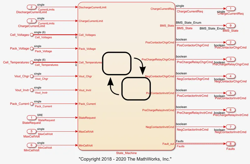
State Machine defines the central operating state of the BMS. The state machine has four parallel states (parallel meaning that they can be active at the same time):

a. The first one defines the variable BMS_State, which indicates standby, driving, charging, and fault. Charging comprises constant current and constant voltage stages.

b. The second state switches the fault state ON if a current, voltage, or temperature value reaches an unsafe level.

c. The third and fourth states define the contactor ON & OFF switching sequence for the charger and inverter. This is needed to avoid a substantial current inrush at the beginning of the charging stage.

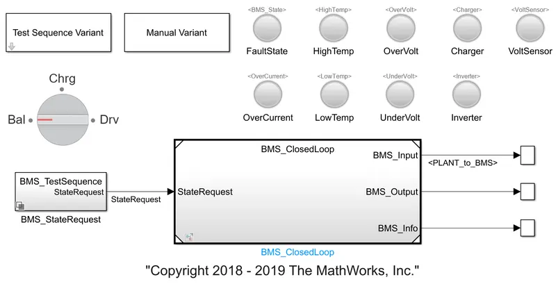
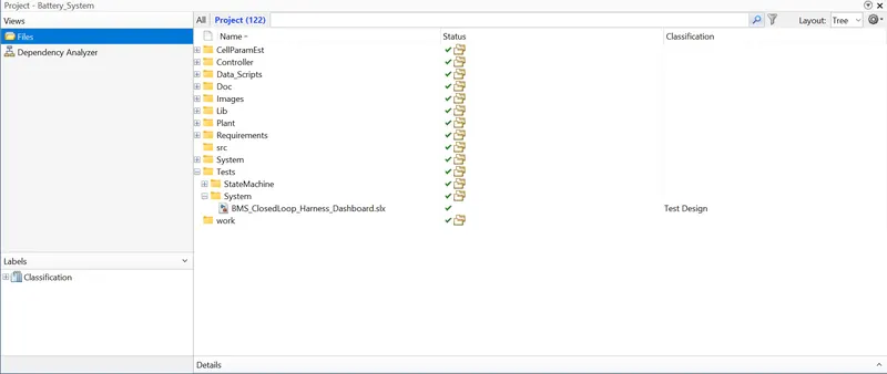
After opening the BMS system, we must go for the harness dashboard. This dashboard can be selected from the MATLAB window following the procedure below.

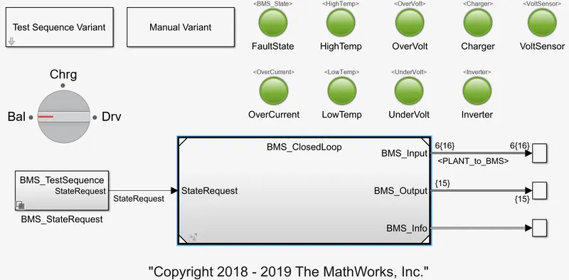
The Harness Dashboard consists of a test sequence variant subsystem with three test cases. This dashboard also helps in determining the fault states and other parameters. The green indicates that the system is working without any error, while the red signal indicates a fault in the system.

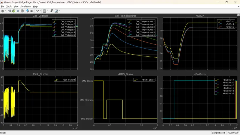
After the successful compilation, the scope opens up. The scope consists of the measurements of cell voltages, cell temperatures, SOC, pack current, and BMS State.

Test Case 1: Now, let's test the 1st test case. Select the Test Sequence Variant and set it to 1. Now run the simulation.

After running the simulation, the dashboard shows a green signal in all the parameters. This indicates that there are no errors or faults.

In this test case, there are three stages of driving condition, namely - 

• Driving
• Charging
• Standby

When the simulation begins, the vehicle is initially driving, and the SOC will decrease for this period. After 3000 seconds, the next step is balancing mode, and the vehicle is in the charging phase, and the battery's SOC increases almost to 100%. The next phase is the post-charging phase, in which the vehicle goes into standby mode again.

Scope Results:

• The input cycle can be seen in the BMS_State plot in which the vehicle initially undergoes driving, then charging till SOC = 90% and later in the standby state.
  
  
• During charging, the battery pack voltage is increased up to 4.2V.
• The cell temperature increases during the driving and charging cycle and starts falling off in the standby mode.
  
  
• The SOC drops to less than 50% after the driving cycle and is then later put into charging until SOC reaches 100%.
  
  
• The current supplied to the EV during the driving phase can be seen in the Current plot.

Test Case 2: Now, let's test the 2nd test case. Select the Test Sequence Variant and set it to 2. Now run the simulation.

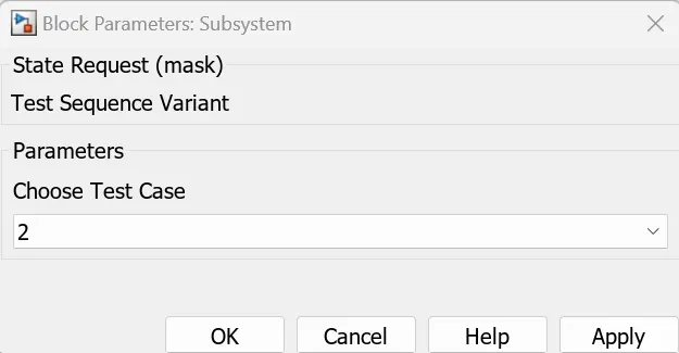
The result shows that there is a fault condition in the vehicle. The dashboard on the model depicts the same with a red colour indication.

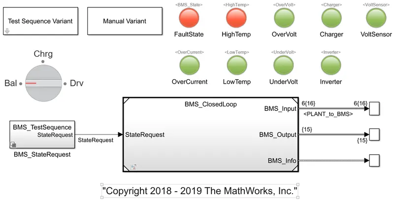
This test case has two phases for the battery pack:

• Driving 
• Charging

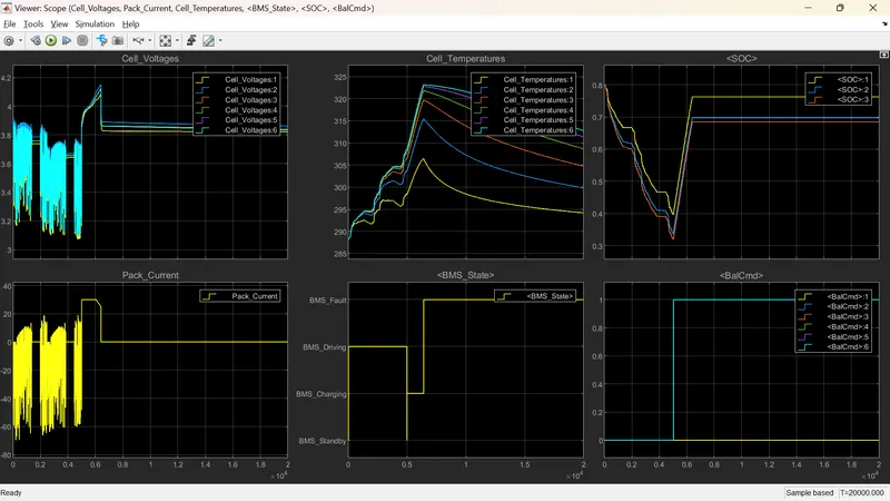
The scope result shows the various parameters for the BMS Model under the second test case. After 10,000 seconds, when the driving cycle is over, the fault condition occurs, and so the SOC does not increase even for the charging phase.

Test Case 3: Now, let's test the 3rd test case. Select the Test Sequence Variant and set it to 3. Now run the simulation.

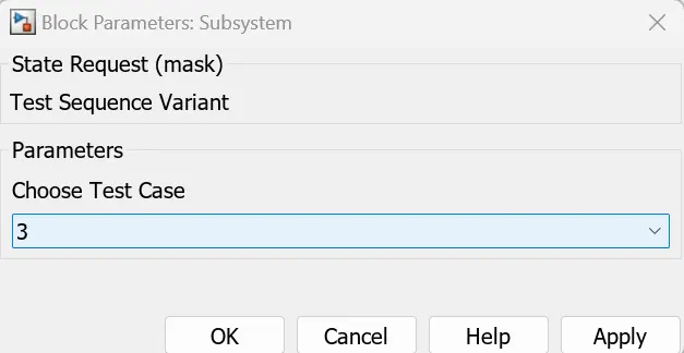
After running the simulation, the dashboard shows no errors or faults.

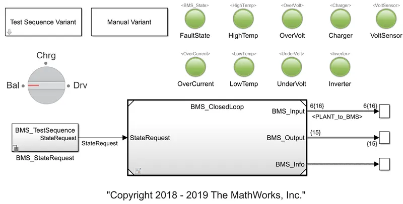
In this test case, only Charging Phase is there.

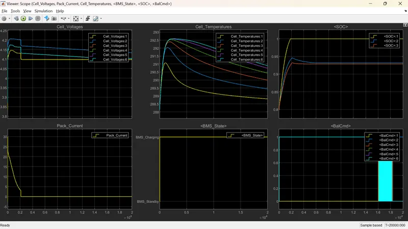
The scope result indicates that the SOC increases from 80-100% and remains in standby mode.

Following these steps, the BMS model can be implemented to check the faults and errors using the three test cases from the harness dashboard.

2. The Coulomb Counting method measures the discharging current of a battery and integrates the discharging current over time to estimate SOC. The Coulomb Counting method estimates the SOC values, which are estimated from the discharging current and previously estimated SOC values.

The following equation calculates SOC:

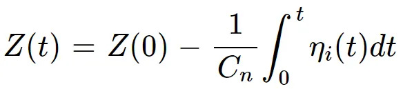
Z(t) = Actual SOC
Z(0) = Initial SOC
Cn = Capacity of the Battery
t = Instantaneous time
i(t) = Instantaneous current

Let us understand further from the Q1 model. 

Select the BMS ECU subsystem.

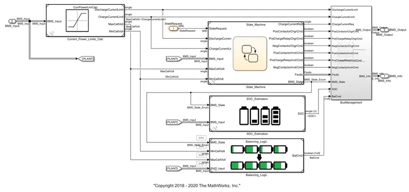
Now, select the SOC Estimation subsystem.

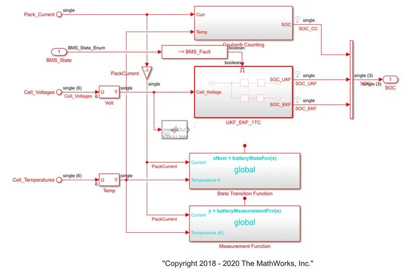
Finally, select the Coulomb Counting subsystem.

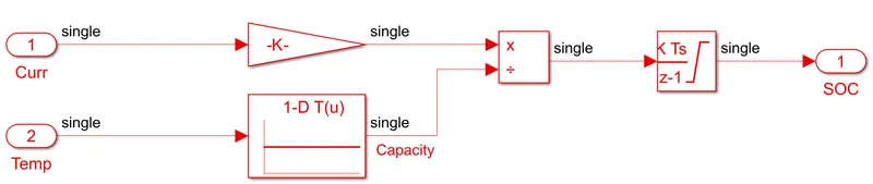
• As the name suggests, this method aims to calculate coulombs or the quantity of electric charge derived from current multiplied by the time necessary for the charge to flow. To measure a battery's remaining capacity or SoC, coloumbs can be added to the initial capacity in case of charging or taken away when the battery gets discharged.
  
  
• The current integration is widespread, but its accuracy depends on some factors. First, we should know the correct measure of the initial SOC that serves as a reference point. We can get this by fully charging or discharging a battery. So if we want to use this technique, We need to allow regular resetting of the battery SOC to 100% in Wer BMS design.
  
  
• Another essential condition for the accurate state-of-charge estimation with coulomb counting is the correct, current measurement. We can achieve this by increasing the amplitude and time resolution of an analogue-to-digital converter (ADC) in your current sensor. However, this can add to the sensor's cost, so in most cases, BMS designers use inexpensive ADCs with 14- and 16-bit resolution and average measured data afterwards. Then, engineers process data by applying more advanced estimators, such as  Kalman filtering or neural networks. 
  
  
• If we can provide the conditions necessary for the efficient use of the current integration method, we can reach high accuracy in our SoC calculation.