Week 7 State of charge estimation
AIM:- To study the state of charge estimation with the help of MATLAB and SIMULINK.
OBJECTIVES:-
1.Simulating the 3 test cases from the harness dashboard and write a detailed report on the results
2.What is coulomb counting? Refer to the above model and explain how BMS implements coulomb counting for SOC estimation?
Q.1.Simulate the 3 test cases from the harness dashboard and write a detailed report on the results
Ans:-
Simulating the 3 test cases from the harness dashboard,'
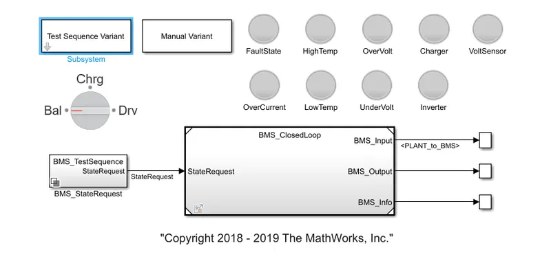
- now we will run the test cases by double-clicking the test sequence variant there are three cases that we will run in sequence
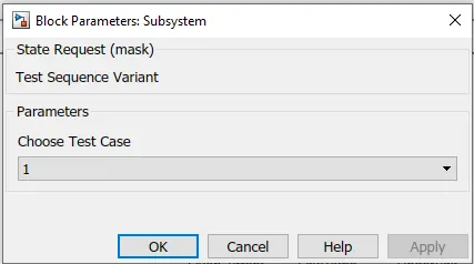
a)by running the simulation we got our first result graph,
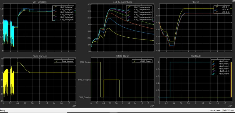
Observation:-As the simulation ends we got 6 result graph considering the BMS is an operation for electrical vehicle
1.the first graph indicates the cell voltage of all the cells involved in the battery pack we first observed that cell voltages changing as the current flowing in and out. at the beginning of the simulation, the voltages are slightly different because we initialize the model with a slight associate of imbalance the voltages are deflecting from the range of 3.1 v to 3.9 volts for the time period of 0.3*10^4 sec, and then there is balances state of all voltage of their respective cells and then there is a sudden hike in cell voltage till they reach 4.2 volts and at the end of the simulation, the values converge towards one another and trying to balance the voltages till the end still there is a small difference in their voltages and the voltage line flows between 4 to 4.2 volt. because the system goes on standby mode.
2.in charging state during the constant current phase current(current is deflecting in the range of 19 A TO -70 for 0.3*10^4 sec) is debated because the maximum cell voltage is high, enough compared to prescribe 4.4-volt limit that an excessively high current control the voltage beyond the threshold significantly limiting the life of the battery
3. 3.the temperature(it's starting from the range of 289-degree Celcius and at the end, all the cells have a different temperature) traces show the significant discrepancy between the hottest and coldest cell the reason is mainly because of symmetry in the merger layer in terms of thermal behavior. the cell no 6 is significantly hotter the cell no 1 because it is thermally insulated on one side. even if the maximum temperature reached during the simulation is not concerned in terms of safety. the temperature difference at cell no 6 at its higher temperature will eventually cost much faster degradation of cell 6 compared to cell 1 leading to undesirable and uneveness in cell condition. therefore need an active thermal management system to keep thermal differences within a few degree Celcius.
4.the graph no 3 show the soc of three different battery cell each performed with different matter yellow corresponds to column counting, blue corresponds to ukf and orange to ekf, the initial soc is 75%, however, the simulation so estimates need to initialize it to 80% to set their capability to recover.it is apparent that columb counting never does because it has no way to realize it is wrong due to the absence of voltage information. both common filter algorithms on the other hand recover from the initial error within the first hour of simulated time. with the ekf slightly outperforming then ukf.
5.the other scopes indicate the bms state at each of the balance command signals respectively.
b)after stimulation of 2nd case of test sequence variant,
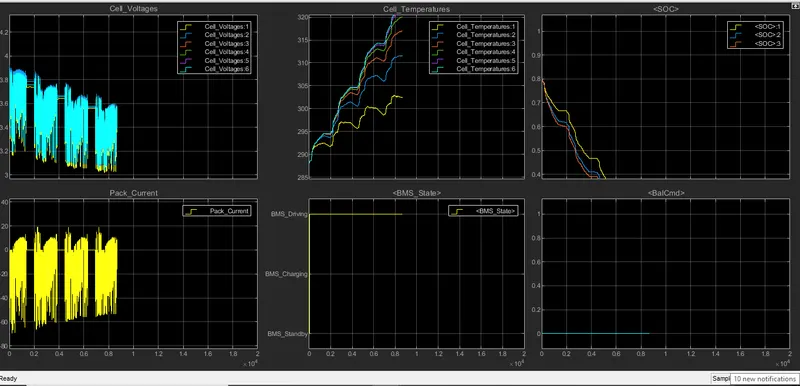
Observations:-
1.at the initial state the voltage of all the cells are deflecting in the same manner and dropping slightly in the range of 3 to 3.9 volt it has 4 fluctuation zones and in between each of these fluctuating zone, they are stable for while and this phase lasts for 0.85*10^4 sec. (throughout the simulation BMS has put on driving mode).
2.on the other hand the current graph has exactly flowed in the same manner but in the opposite direction when voltage is getting drop current required is high and current flows in the range of -70 A to 20 A.
3.the temperature of all the cells initiating from 288-degree Celcius and they get scattered all the cells have a different temperature) traces show the significant discrepancy between the hottest and coldest cell the reason is mainly because of symmetry in the merger layer in terms of thermal behavior. cell no 6 is significantly hotter the cell no 1 because it is thermally insulated on one side. even if the maximum temperature reached during the simulation is not concerned in terms of safety.
4. the cells are initially at 80% of soc and then they're falling at different time periods. to set their capability to recover.it is apparent that columb counting never does because it has no way to realize it is wrong due to the absence of voltage information. both common filter algorithms on the other hand recover from the initial error within the first hour of simulated time. with the ekf slightly outperforming then ukf then is apparent that columb counting never does because it has no way to realize it is wrong due to the absence of voltage information. both common filter algorithms on the other hand recover from initial error within the first hour of simulated time. with the elf slightly outperforming the ukf.
5.the other scopes indicate the bms state at each of the balance command signals respectively. where it's on driving mode and command signals on zero lines.
c)after simulation of 3rd case of test sequence variant,
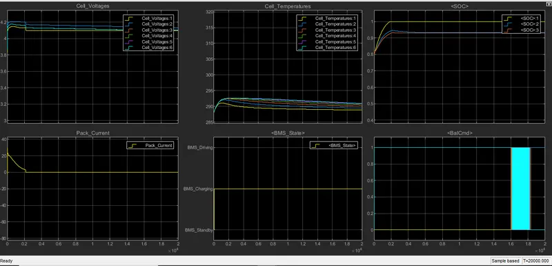
Observations:-
1.all the cells are initiated with at different voltages the where the 6 the one having the higher voltage of 4.2 volts and the 1st one having near about 4.1 v and remaining falling under this range BMS on charging state throughout the simulation. so the voltage graph move along in a straight line because the voltage supply continues .there have some deflection of voltage lines of different cells but that is a very less amount of change in voltage .at the end of the simulation BMS trying to balance the voltage very much
2.the battery pack current is initiated with 20 A and then it falls to zero current till its complete simulation time of 0.2*10^4 sec and then it maintains the constant current because it is put on charging state and it remains constant throughout the simulation
3.all the cells initiate with 287-degree Celcius and then all the cells maintaining the straight line but with different temperatures range. the end all the cells have a different temperature) traces show the significant discrepancy between the hottest and coldest cell the reason is mainly because of symmetry in the merger layer in terms of thermal behavior. cell no 6 is significantly hotter the cell no 1 because it is thermally insulated on one side. even if the maximum temperature reached during the simulation is not concerned in terms of safety. the temperature difference at cell no 6 at its higher temperature will eventually cost much faster degradation of cell 6 compared to cell 1 leading to undesirable and unevenness in cell condition. therefore need an active thermal management system to keep thermal differences within a few degree Celcius.
4.the soc is initial soc of three different cells is at 80% as the. as the system is put on charging state the soc hikes up to 100% for the yellow cell,ukf and ekf initially having different charging rates but after 0.4*10^4 sec they having equal state of charge of 91% and it maintains throughout the simulation .t is apparent that columb counting never does because it has no way to realize it is wrong due to the absence of voltage information. both common filter algorithms on the other hand recover from the initial error. ekf and urf slightly outperforming then coulomb counting.
5. the other scopes indicate the bms state at each of the balance command signals respectively. bms on charging state and battery command passing signal between 0 to 1.
Q.2.What is coulomb counting? Refer to the above model and explain how BMS implements coulomb counting for SOC estimation?
Coulomb Counting Method
The Coulomb counting method measures the discharging current of a battery and integrates the discharging current over time to estimate SOC. Coulomb counting method is done to estimate the SOC(t), which is estimated from the discharging current, I(t), and previously estimated SOC values, SOC(t-1). SOC is calculated by the following equation:
a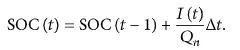
But several factors affect the accuracy of the Coulomb counting method including temperature, battery history, discharge current, and cycle life.
Modified Coulomb Counting Method
To improve the Coulomb counting method, a new technique called the modified Coulomb counting method is proposed. The modified Coulomb counting method uses the corrected current to improve the accuracy of estimation.
The corrected current is the function of discharging current. There is a quadratic relationship between the corrected current and discharging current of the battery. By the practice of experimental data, the corrected current is calculated by the following form:

where K1, K2, and K0 are constant values obtained from the practice experimental data.
In the modified Coulomb counting method, SOC is calculated by the following equation:
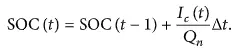
The experimental results show that the accuracy of the modified Coulomb counting method is superior to the conventional Coulomb counting method.
Flowchart for columb counting
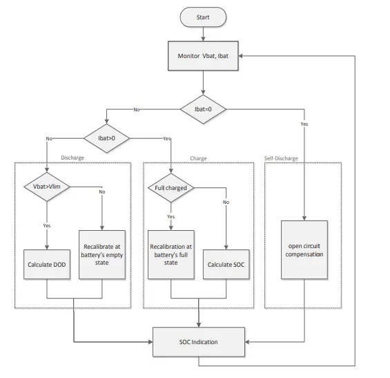
The flowchart given in Fig.3 explains the algorithm used to manage the battery monitoring by switching from a battery operating mode to another by the conditions of the transition
The estimation of the SOC of a Li-Ion battery in this method is based on monitoring both the voltage ܸVbat and the current Ibat. The operation mode of the battery is recognized by the direction of current through the battery system.
When the battery is in open circuit mode, Ibat = 0 and compensation of self-discharge losses will be taken into account as explained in sub-section C.
The information needed to carry monitoring is the measurement of the battery voltage, the current flowing
through it, and the operating temperature. Coulomb counter ∆ܳQ is used to track the SOC when the battery is charged or discharged.
The amount of charges ∆ܳQ in an operating period 'τ' is obtained by temporal integration of a measured charging/discharging current Ibat like expressed in (2)

This variance ∆ܳQ that will be used in the following equations is negative if the battery is in discharge, positive if in charge.
A. Charge Mode
In this mode, the coulomb counter is presented by ܳQgained as expressed in (3), which represents the number of charges accumulated during 'τ'

So the variation of the state of charge gained in this same operating period is obtained by the relation (4)

By cumulating the previous state of charge indication and the obtained one we can have the instantaneous value of ܱܵSOC.

Knowing the relationship indicated about (6) the value of depth of discharge DOD is updated in every charging operation to get it back every switching to discharging mode.

B. Discharge Mode
In the discharging mode the coulomb counter is presented by Qlost, which represents the amount of charges losses in the operating period 'τ' by equation (7):

The depth of discharge variation is calculated according to (8) and used in (9) to calculate the value of DOD


The SOC indication then is done by applying the equation (6).
C. Self-Discharge Mode
At the battery storage periods, the percentage of monthly self-discharge is converted to the amount discharged per hour; this amount is designed by the constant q(per/hour). Considering a 5% rate of self-discharge per month q(per/hour) is approximated to 0.0016 Ah. So the quantity of charges dissipated in the open circuit period ܳQoc is calculated by equation (10) representing the accumulative losses during the store hours.

ℎ: Hour of storage
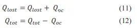
This value will be added to the amount of charge lost ܳQlost during discharge mode and subtracted from the amount of charge accumulated ܳQgained in charge mode as expressed in relations (11) and (12). This compensation of self-discharging loss is made at each open circuit period and before switching to
another operating battery’s mode.
D. Temperature effect
The temperature variation affects considerably the state of charge of the Li-Ion battery [16]. To improve the accuracy of the battery state of charge, a temperature coefficient ߙ is introduced and multiplied by the value of the calculated SOC [17]. This coefficient varies depending on the operating temperature according to the intervals variations (13)

E. Recalibration
When the loaded voltage ܸVbat drops under a limit voltage Vlim (3V), during the discharging mode the battery is considered totally discharged. When it’s empty, the battery can no longer be used and should be recharged. So after a cycle of charge/discharge, a recalibration should be made of Qmax which represents the maximum capacity that can be released by the battery. This recalibration allows rectifying the
indication of SOC by replacing ܳQrated by Qmax in relation (4). Also, we recalibrate the State-of-Health (SOH) of the battery SOH defined is a relation (14) as:

Moreover, the battery is fully charged. Then ܱܵSOH should be updated by assigning the number of charges releasable from the battery to Qmax. The SOH indeed represents the aging degree of the battery; in fact, it’s at 100% maximum value when the battery is new. When the battery is getting old and ܳQmax became more and more inferior than ܳQrated, SOH value drops to indicate the health degradation of the battery.
Refer to the above model and explain how BMS implements coulomb counting for SOC estimation?
Ans:-
this model contains BMS ECU and PLANT to calculate estimate soc of battery management system we need to enter the plant block
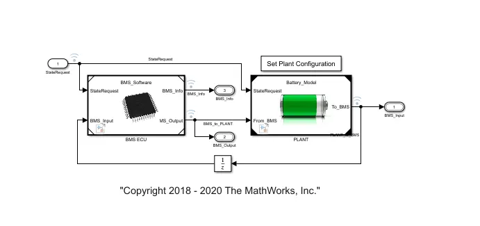
-before we charge our vehicle we need an accurate Estimation of battery SOC, in the battery system we don't measure the state of charge we measure different things like battery pack current cell voltage and cell voltage which we taking signals as input from the plant.
-after entering the plant block we can see the state machine, SOC estimation, and balancing logic block
-in which we going to study SOC estimation.
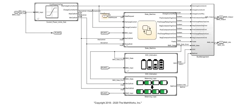
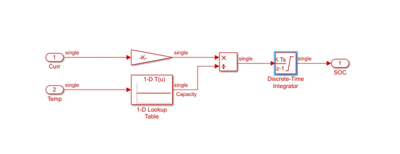
-in this SOC estimation block we can see three different techniques for the state of charge estimation. all three techniques have their own merits and limitations. the first method is columb counting and the other two are unscented(ukf) and extended Kalman filter(ekf).here we are concern with the columb counting method.
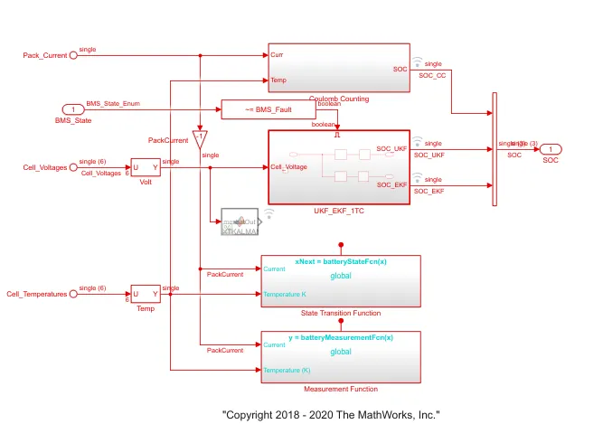
-in coulomb counting method block
-it takes two input signals such as current and temp and the current signal goes to gain block and the temp signal goes to lookup tables of battery time and current. and both the blocks are connected to the divided block and these signals are connected to the discrete-time integrator to track the charge and which finally helps to calculate the state of charge.
-which consist of integrating a current and doesn't leave the cell for that here we using discrete-time integrator to give the track of the cell charge of the time the benefits of this is its simplicity and its low capitation cost and the drawbacks are an accumulation of current sensor error and its inability to recover from the wrong initial condition. from the lack of feedback from voltage measurements.
*************************************************************************************
CONCLUSIONS:-
1)one of the main problems in coulomb counting is that it is necessary to calibrate the initial battery SOC. In several applications, the initialization involves rest and the initial SOC is estimated based on the voltage
2)Kalman filtering is an algorithm that provides estimates of some unknown variables given the measurements observed over time.
REFERENCES:-
1)https://www.mathworks.com/videos/series/how-to-develop-battery-management-systems-in-simulink.html