Project 2 - Rankine cycle Simulator
AIM:- To simulate rankine cycle by using MATLAB.
OBJECTIVES:-
1)To calculate the state points and display them in command window.
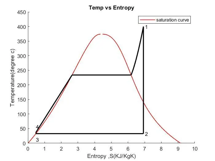
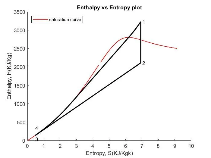
2) To plot the corresponding T-s and h-s for given set of inputs.
THEORY:-
The Rankine cycle or Rankine Vapor Cycle is the process widely used by power plants such as coal-fired power plants or nuclear reactors. In this mechanism, a fuel is used to produce heat within a boiler, converting water into steam which then expands through a turbine producing useful work. This process was developed in 1859 by Scottish engineer William J.M. Rankine.This is a thermodynamic cycle which converts heat into mechanical energy—which usually gets transformed into electricity by electric generation.
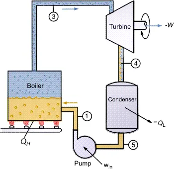
Fig 1.1 Rankine cycle schematic diagrm
Basic Cycle
The Rankine cycle is the fundamental operating cycle of all power plants where an operating fluid is continuously evaporated and condensed. The selection of operating fluid depends mainly on the available temperature range.
The pressure-enthalpy (p-h) and temperature-entropy (T-s) diagrams of this cycle are given in . The Rankine cycle operates in the following steps:
-
1-2-3 Isobaric Heat Transfer. High pressure liquid enters the boiler from the feed pump (1) and is heated to the saturation temperature (2). Further addition of energy causes evaporation of the liquid until it is fully converted to saturated steam (3).
-
3-4 Isentropic Expansion. The vapor is expanded in the turbine, thus producing work which may be converted to electricity. In practice, the expansion is limited by the temperature of the cooling medium and by the erosion of the turbine blades by liquid entrainment in the vapor stream as the process moves further into the two-phase region. Exit vapor qualities should be greater than 90%.
-
4-5 Isobaric Heat Rejection. The vapor-liquid mixture leaving the turbine (4) is condensed at low pressure, usually in a surface condenser using cooling water. In well designed and maintained condensers, the pressure of the vapor is well below atmospheric pressure, approaching the saturation pressure of the operating fluid at the cooling water temperature.
-
5-1 Isentropic Compression. The pressure of the condensate is raised in the feed pump. Because of the low specific volume of liquids, the pump work is relatively small and often neglected in thermodynamic calculations.
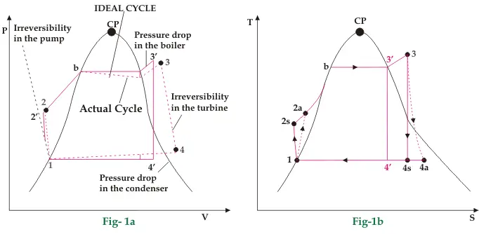
What is the ideal vs actual rankine cycle?
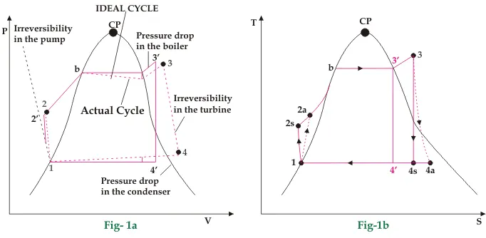
fig 1.2 Ideal vs actual rankine cycle
Energy balance for the actual Rankine Cycle is as follows:
| Actual Rankine Cycle Components | Heat | Work |
| Boiler feed Pump Wpump-in |  |
 |
| Boiler |  |
 |
| Turbine | |
 |
| Condenser |  |
|
| Thermal efficiency of Ideal Rankine cycle |  |
 |
CODE:-
-Writing a matlab code to simulate rankine cycle and plotting graph for h-s and t-s
clear all
close all
clc

disp('                RANKINE CYCCLE           ')

disp('1-2 is Isentropic Expansion in the Turbine');
disp('2-3 constant pressure heat rejection by condensor');
disp('3-4 is Isentropic Expansion in the pump');
disp('4-1 constant pressure heat addition to the boiler');

%inputs:
disp('               INPUTs                     ')
P1 = input('Enter the pressure at turbine inlet(bar):');
T1 = input('Enter the temperature at the turbine inlet(degree C):');
P2 = input('Enter the pressure at the condensor(bar):');

%using the Xsteam  functions,the enthalpy and entropy at various state can
%be calculated

%calculating enthaloy(h) and entropy(s)at point 1
h1 = XSteam('h_pT',P1,T1);
s1 = XSteam('s_pT',P1,T1);

%calculating pressure(P),enthalpy(h) and entropy(s)at point 2

%since isentropic exapansion :-
s2=s1;
sf2=XSteam('sL_P',P2);
sg2=XSteam('sV_P',P2);
x2=(s2-sf2)/(sg2-sf2);
hf2=XSteam('hL_P',P2);
hg2=XSteam('hV_P',P2);
h2=hf2+(x2*(hg2-hf2));


%Calculating pressure(P),enthalpy(h) and entropy(s) at point 3;

%since constant pressure heat removel:
P3=P2;
h3 = XSteam('hL_P',P3);
s3 = XSteam('sL_P',P3);

%Calculating pressure(P),enthalpy(h) and entropy(s) at point 4:

%since iscentropic compression:
s4=s3;

%since constant pressure process:
P4=P1;
%%%%
%work done by turbine
Wt = h1-h2;

%work done by pump
V3 = XSteam('vL_P',P3);
Wp = V3*(P4-P3)*100;
h4 = h3 + Wp;

%net work
Wnet = Wt-Wp;

%Heat into the system
Qin = h1-h4;

%heat out of the system
Qout = h2-h3;

%Thearmal efficiency
eff = (Wnet/Qin)*100;

%specific steam consumption
%SSC = mass flow rate/power
SSC=(3600/Wnet);

%calculating temperature at the state points
T3 = XSteam('Tsat_P',P3);
T2=T3;
Cp4 = XSteam('Cp_ps',P4,s4);
Cv4 = XSteam('Cv_ps',P4,s4);
k = Cp4/Cv4;
T4 = T3/((P3/P4)^((k-1)/k));

%calculating temperature,entropy and enthalpy at the vapour and liquid
%line for plotting
T6 = XSteam('Tsat_P',P1)
s5 = XSteam('sL_P',P1);
s6 = XSteam('sV_P',P1);
h5 = XSteam('hL_P',P1);
h6 = XSteam('hV_P',P1);
T5=T6;


%calculating entropy and enthalpy at the saturation curve:
 T = linspace(1,375,1000);
  for i = 1:length(T);

  sg(i) = XSteam('sV_T',T(i));
  sf(i) = XSteam('sL_T',T(i));


  hg(i) = XSteam('hV_T',T(i));
  hf(i) = XSteam('hL_T',T(i));

  end

  %Plotting T-s diagram
  figure(1)
  hold on
  plot(sf,T,'r','linewidth',1)
  plot(sg,T,'r','linewidth',1)
  plot([s1 s2],[T1 T2],'k','linewidth',2)
  plot([s2 s3],[T2 T3],'k','linewidth',2)
  plot([s3 s4],[T3 T4],'k','linewidth',2)
  plot([s4 s5],[T4 T5],'k','linewidth',2)
  plot([s5 s6],[T5 T6],'k','linewidth',2)
  sc1 = linspace(s6,s1,1000);
  for l=1:length(sc1);
      Tc1(l) = XSteam('T_ps',P1,sc1(l));
  end

  plot(sc1,Tc1,'k','linewidth',2)
  text(s1+0.1,T1,'1')
  text(s2+0.1,T2,'2')
  text(s3,T3-20,'3')
  text(s4,T4+20,'4')
  title('Temp vs Entropy')
  xlabel('Entropy ,S(KJ/KgK)')
  ylabel('Temperature(degree c)')
  legend('saturation curve')

  %plotting h-s diagram
  figure(2)
  hold on
  plot(sf,hf,'r','linewidth',1)
  plot(sg,hg,'r','linewidth',1)
  plot([s1 s2],[h1 h2],'k','linewidth',2)
  plot([s2 s3],[h2 h3],'k','linewidth',2)
  plot([s3 s4],[h3 h4],'k','linewidth',2)
  hc = linspace(h4,h5,100);
  for k=1:length(hc);
      sch(k) = XSteam('s_ph',P1,hc(k));
  end
  plot(sch,hc,'k','linewidth',2)
  plot([s5 s6],[h5 h6],'k','linewidth',2)
  for m=1:length(sc1);
      hc1(m) = XSteam('h_pS',P1,sc1(m));

  end
  plot(sc1,hc1,'k','linewidth',2)
  text(s1+0.1,h1,'1')
  text(s2+0.1,h2,'2')
  text(s3,h3-100,'3')
  text(s4,h4+200,'4')
  title('Enthalpy vs Entropy plot')
  xlabel('Entropy, S(KJ/Kgk)')
  ylabel('Enthalpy, H(KJ/Kg)')
  legend('saturation curve','location','northwest')


 %state variables at state point 1
 disp('RESULTS');
 fprintf('At state point 1:\n')
 fprintf('P1: %8.3f bar\n',P1);
 fprintf('T1: %8.3f C\n',T1);
 fprintf('h1: %8.3f KJ/Kg\n',h1);
 fprintf('s1: %8.3f KJ/KgK\n',s1);

 fprintf('At state point 2:\n')
 fprintf('P2: %8.3f bar\n',P2);
 fprintf('T2: %8.3f C\n',T2);
 fprintf('h2: %8.3f KJ/Kg\n',h2);
 fprintf('s2: %8.3f KJ/KgK\n',s2);
 fprintf('x2: %8.3f \n',x2);

 fprintf('At state point 3:\n')
 fprintf('P3: %8.3f bar\n',P3);
 fprintf('T3: %8.3f C\n',T3);
 fprintf('h3: %8.3f KJ/Kg\n',h3);
 fprintf('s3: %8.3f KJ/KgK\n',s3);

 fprintf('At state point 4:\n')
 fprintf('P4: %8.3f bar\n',P4);
 fprintf('T4: %8.3f C\n',T4);
 fprintf('h4: %8.3f KJ/Kg\n',h4);
 fprintf('s4: %8.3f KJ/KgK\n',s4);

 fprintf('Turbine work: %8.3f KJ/Kg\n',Wt);
 fprintf('Pump work: %8.3f KJ/Kg\n',Wp);
 fprintf('Wnet: %8.3f KJ/Kg\n',Wnet);
 fprintf('Efficiency: %8.3f percent\n',eff);
 fprintf('S.S.C: %8.3f KJ/Kw\n',SSC);
GRAPHS:-
1)plotting a graph of temperature vs entropy
2)plotting a graph of enthalpy vs entropy:-
-steps that we followed to execute the code-
1)starting with close all,clear all and clc command to erase all previous file residuals.
2)then displaying all the process in command window which are taken place during rankine cycle with disp command.
3)then displaying all the initial state vairable inputs in command window with the help of display command.
4)then introducing xsteam function into the program to calculate state variables.
5)to use xsteam function in program the xteam liabrary file must be present in same folder where our code is saved.
6)then calculated enthalpy and entropy at state point 1
7)then calculating state point 2 variables since the state 2 process is isentropic compression so calculating enthalpy and entropy for gaseous state and fluid state of working fluid with the help of xsteam function
8)after that calculating state variables for state point 3 which is constant pressure heat removel
9)then calculating pressure,enthalpy and entropy at state point 4,where entropy of state point 3 is equal to state point four and since constant pressure so P4=P1.
10)then calculated work done by turbine and pump and net work output.
11)then calculated the heat entered into the system and heat removed from the system.
12)the calculated thermal efficiency of the rankine cycle and specific steam consumption.
13)the calculating the temperatures at state points.
14)then calculating the temperature,enthalpy and entropy at vapour and liquid state.
15)then calculating enthalpy and entropy at saturation curve.
16)then plotting ts diagram with the help of temperature and entropy values at all states which we calculated.
16)then plotting hs diagram with the help of enthalpy and entropy values at all states which we calculated.
17)then displaying all the outputs in the command window with the help of printf command
and by running code we got all the outputs and graphs.
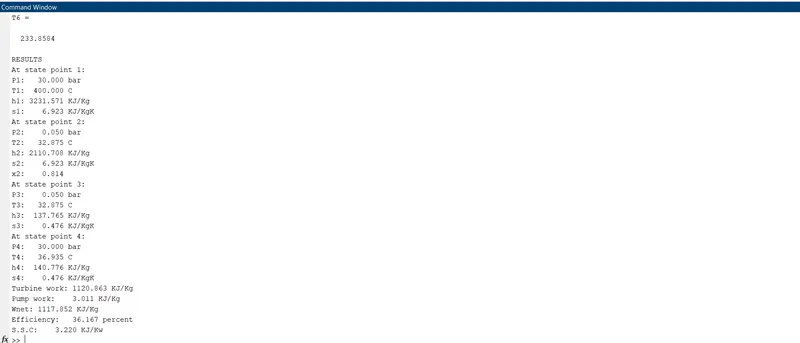
outputs display in the command window:-
RESULTS:-
1) NET WORK OUTPUT:- 1117.852 KJ/Kg
2) EFFICIENCY OF RANKINE CYCLE:- 36.167%
CONCLUSION:-
The overall effect of lowering the condenser pressure is an increase in the thermal efficiency of the cycle.
REFERENCES:
1)Fig no 1.1 is taken from:-http://thermopedia.com/content/5493/927RCFig1.gif

2)Fig no 1.2 is taken from:-https://www.electrical4u.com/images/september16/1479300944.png
(Note:- All the related screenshots are attach below)