Week 3 - Solving second order ODEs

AIM:- Write a program that simulate motion of pendulum by using MATLAB with the help of givevn 2nd ODE.

OBJECTIVES:-

1) To plot graph of displace and velocity vs time where we are going to observe how damping factor is going to change nature of velocity and displacement waves.

2) Creating a animation video of simple pendulum for a time span.

INTRODUCTION:-

WHAT IS SIMPLE PENDULUM?

A point mass attached to a light inextensible string and suspended from fixed support is called a simple pendulum. The vertical line passing through the fixed support is the mean position of a simple pendulum.

The vertical distance between the point of suspension and the centre of mass of the suspended body (when it is in mean position) is called the length of the simple pendulum denoted by L.

DIGRAM:-

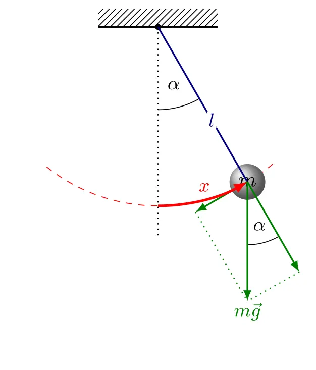
FIG 1.1-SIMPLE PENDULUM

where,

m - mass of spherical ball in 'kg'

g - gravitty along the mass in 'm/s^2'

l - length of pendulum string in 'm'

b - damping coefficient

APPLICATION OF SIMPLE PENDULUM:-

Pendulums are in common usage. Some have crucial uses, such as in clocks; some are for fun, such as a child's swing; and some are just there, such as the sinker on a fishing line. For small displacements, a pendulum is a simple harmonic oscillator.

-we are going to solve simple pendulum problem which is represented by 2nd ODE

A second order ordinary differential equation is an ordinary differential equation in which any derivatives with respect to the independent variable have order no greater than 2.

PROBLEM :-

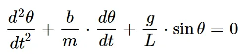
-this is 2nd ODE which represent simple pendulum we need to solve the ode to write program.

Given data:-

L = 1 metre.

m = 1 kg.

b = 0.05

g = 9.81 m/s^2

simulate the motion between 0-20 sec,for angular displacement=0,angular velocity=3 rad/sec at t=0.

SOLUTION :-

first we are going to convert our 2nd order degree equation into set of 1st order degree equation,

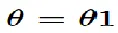..... theta=theta1

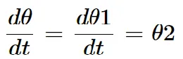...... (1)equting theta = theta 1

..........(2)

.........equating theta = theta1 into original equation

...................from equation no 2

we finally got two equation wgich are elements of matrix

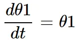..............................(1)

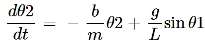.............(2)

as we got elements of matrix now will solve this in matlab

CODE:-

in first half we are going to define function and writing program for that,

function [dtheta_dt] = ode_func(t,theta,b,g,l,m)
        theta1 = theta(1);
        theta2 = theta(2);
        dtheta1_dt = theta2;
        dtheta2_dt = -(b/m)*theta2-(g/l)*sin(theta1);
        dtheta_dt = [dtheta1_dt; dtheta2_dt];
 
end       

1. first we define our ode function and for that we are writing this code seprately which will help us in final program. assigning the same file name similer to our ode function.
2. ode_func cobtains time ,theta ,damping coeff,length,mass as inputs.
3. then we are defining theta1 and theta2 which is our solution array which we solved above.
4. then we defined our both ode's which are dtheta1_dt and dtheta2_dt.
5. then we combines both the odes into a array which is dtheta_dt
6. and seprated both the ode's with semicolon that means we have two rows
7. finnly this function will gives us outout in the final program which will be column vector containing two results.

-in second half we are going to plot the graph of velocity and disp vs time and also make a animation video of simple pendulumC

CODE:-

clear all
close all
clc

%solving second order diffrential equation which represent the motion of
%simple pendulum and damping effect

%given data
g = 9.81;      % gravity in 'm/s^2'
l = 1 ;        % length of the pendulum in 'm'
m = 1;         % mass of the ball in 'kg'
b = 0.05;      % damping coefficient

%initial condition when t=0
theta_0 = [0;3];    %ang disp= 0;ang velo=3

%using linspace command to divide o to 20 sec time span in equal parts 
t_span = linspace(0,20,500);

% we are using ode45 solver
[t,results] = ode45(@(t,theta)ode_func(t,theta,b,g,l,m),t_span,theta_0);

%plotting the graph of time vs displace and velocity
figure(1)
hold on
plot(t,results(:,1),'linewidth',2)
plot(t,results(:,2),'linewidth',2)
title('Simple harmonic motion of pendulum')
xlabel('Time(sec)')
ylabel('plot(displacement and velocity)')
legend('Angular displacement','angular velocity')
grid on
hold off

%using a for loop command to repeatedly execute a block of code for animatn
%first of all we are going to our initiat counter is to
theta2 = results(:,1);
ct=1;
for i = 1:length(theta2);    %results(:,1)bcz it includes ang displacement values
   theta_a = theta2(i)
    x0 = 0;                   %intial ang disp of pendulum(x and y)
    y0 = 0;
    
    x1 = l*sin(theta_a)      %final ang disp of pendulum(x,y)
    y1 = -l*cos(theta_a)
    
    %creating animation of simple pendulum
    figure(2)
    plot([-1 1],[0 0],'color','b','linewidth',3);  %for fixed part
    hold on
    plot([x0 x1],[y0 y1],'color','y','linewidth',2);   %for pendulum string
    hold on
    plot(x1,y1,'o','markers',20,'markerfacecolor','r') %for spherical ball
    grid 
    axis([-1.5 1.5 -1.5 1]);   %fixing axis
    pause(0.002)               %using pause command for smooth animation
    hold off
    M(ct) = getframe(gcf);
   
    ct = ct+1;
end    
%creating movie and video file 
movie(M)
videofile = VideoWriter('ode_simple_pendulum.avi','uncompressed AVI');
open(videofile)
writeVideo(videofile,M)
close(videofile)

GRAPH:-

- graph shows simple harmonic motion of simple pendulum for the interval of time 0-20 sec

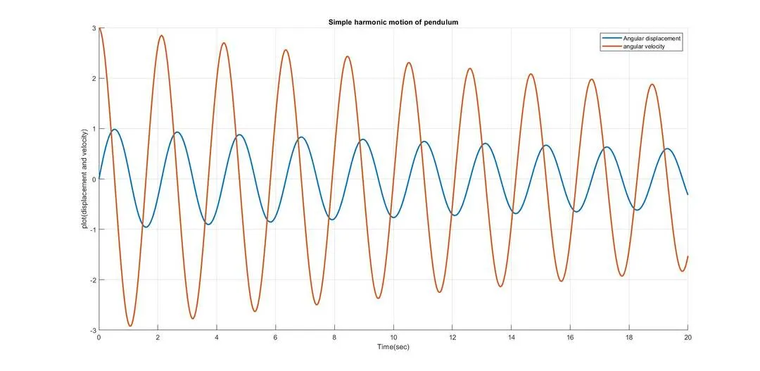
Graph of simple harmonic motion of simple pendulum

-steps that we followed to execute the code

1)first we used clear all,close all and clc command to wiped out prvious data if in case its present.

2)the we entered input parameters which are given .

3)then we set initial condition of velocity and displacement when t=0.

4)then we divide the time span of 0-20 int0 500 equal space intervals with linspace command.

5)then to achieve the output of [t,results] we used ode45 which is inbuild solver

6)then we define that our ode is function of (t,theta)

7)then we are passing input parameters to ode_func and then we provide initial condition after that integration and time array and initial conditions corresponing to starting of time

8)we got two columns which contains values of velocity and displacement from that we can plot graph where time varries from 0-20 and with that disp and velocity values are also changes,which results in shm of simple pendulum

9)after that we are going to animate the motion of pendulum for that we are using for loop command which help us to execute the block of code repeatedly

10)before that we are going to mention our counter is ct= 1

11)then going to decide length of code,initial condition and final condition displacement of of pendulum

12)then we are going to create animation for that we are allocating position ,diamensions and colors of our simple pendulum for spherical ball we used marker command 'o'

13)then we fixed the axis and give a paused to animation with certain value

14)then captured the frame and set our counter value ct=ct+1 so it will increment the frame with +1 everytime

15)the we made a movie of animation with movie command then we saved the movie with similer to file name in 'avi' format and gave location

16)then write the video,open video and finally close the video

17)thats how we executed the code to create animation of simple pendulum

ERRORS:-

-mention linewidth of pendulum with inverted commas and because of that matlab throwing error saying 'value not a numeric scaler' so to rectify this error simply removed the inverted commas and code got executed.(the screenshot of showing error in command window is attached below )

RESULT:-

1) we sucessfully plot graph of angular velocity and angular displacement vs time.

2) sucessfully created a animated video of showing motion of simple pendulum (youtube video link given below)

CONCLUSION:-

By increasing damping coefficient we can damped out maximum oscillations.

REFRENCES :-

1) fig no 1.1 is taken from :-

https://www.teachengineering.org/lessons/view/cub_pend_lesson01

2) for animation of simple pendulum youtube video link is give below:-

https://www.youtube.com/watch?v=RXxzl9lUyw8

(Note:- all the required screenshots are attached below)