Challenge

Week 4 - Genetic Algorithm

AAniket Khedekar27 Dec 2020

AIM:- To write a program in MATLAB to optimize stalagmite function and fine the global maxima of the function with the help of a genetic algorithm.

OBJECTIVES:-

1) to create a customize function for stalagmite in MATLAB.

2) to find global maxima for unbounded inputs.

3) to find global maxima for bounded inputs.

4) to find global maxima for bounded inputs with increasing population size.

THEORY:-

INTRODUCTION:-

1)GENETIC ALGORITHM

2)STALGAMITE

Genetic algorithm:-

Let’s start with the famous quote by Charles Darwin:

"It is not the strongest of the species that survives, nor the most intelligent , but the one most responsive to change."

You must be thinking what has this quote got to do with genetic algorithm? Actually, the entire concept of a genetic algorithm is based on the above line.

Let us understand with a basic example:

Let’s take a hypothetical situation where, you are head of a country, and in order to keep your city safe from bad things, you implement a policy like this.

You select all the good people, and ask them to extend their generation by having their children.
This repeats for a few generations.
You will notice that now you have an entire population of good people.

Now, that may not be entirely possible, but this example was just to help you understand the concept. So the basic idea was that we changed the input (i.e. population) such that we get better output (i.e. better country).

Now, I suppose you have got some intuition that the concept of a genetic algorithm is somewhat related to biology. So let’s us quickly grasp some little concepts, so that we can draw a parallel line between them.

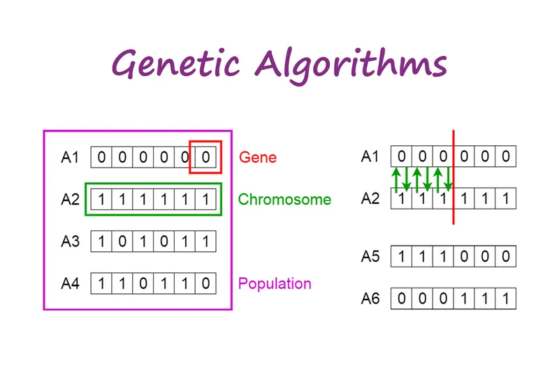
11 Fig 1.1 :-GENETIC ALGORITHM

The notion of natural selection:-

The process of natural selection starts with the selection of the fittest individuals from a population. They produce offspring which inherit the characteristics of the parents and will be added to the next generation. If parents have better fitness, their offspring will be better than parents and have a better chance at surviving. This process keeps on iterating and at the end, a generation with the fittest individuals will be found.

This notion can be applied to a search problem. We consider a set of solutions for a problem and select the set of best ones out of them.

Five phases are considered in a genetic algorithm.

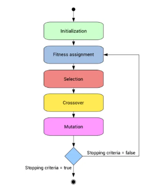
Fig 1.2:-working on genetic algorithm

1)Initial population

The process begins with a set of individuals which is called a Population. Each individual is a solution to the problem you want to solve.

An individual is characterized by a set of parameters (variables) known as Genes. Genes are joined into a string to form a Chromosome (solution).

In a genetic algorithm, the set of genes of an individual is represented using a string, in terms of an alphabet. Usually, binary values are used (strings of 1s and 0s). We say that we encode the genes in a chromosome.

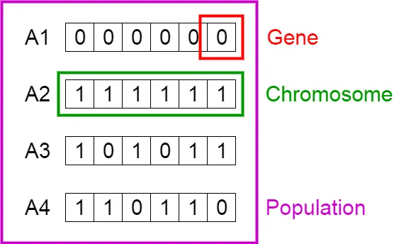
Fig 1.3:-Initial population

2)Fitness function

The fitness function determines how fit an individual is (the ability of an individual to compete with other individuals). It gives a fitness score to each individual. The probability that an individual will be selected for reproduction is based on its fitness score.

3)Selection

The idea of selection phase is to select the fittest individuals and let them pass their genes to the next generation.

Two pairs of individuals (parents) are selected based on their fitness scores. Individuals with high fitness have more chances to be selected for reproduction.

4)Crossover

Crossover is the most significant phase in a genetic algorithm. For each pair of parents to be mated, a crossover point is chosen at random from within the genes.

For example, consider the crossover point to be 3 as shown below.

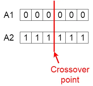
Fig 1.4:-Crossover

Offspring are created by exchanging the genes of parents among themselves until the crossover point is reached.

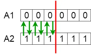
Fig 1.5.1:- Offring

The new offspring are added to the population.

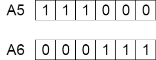
Fig 1.5.2:- Offring

5)Mutation

In certain new offspring formed, some of their genes can be subjected to a mutation with a low random probability. This implies that some of the bits in the bit string can be flipped.

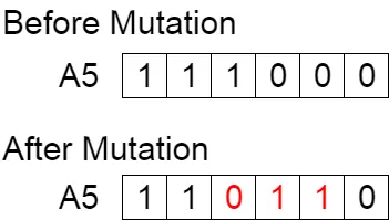
Fig 1.6:-Mutation

A mutation occurs to maintain diversity within the population and prevent premature convergence.

4)Termination

The algorithm terminates if the population has converged (does not produce offspring which are significantly different from the previous generation). Then it is said that the genetic algorithm has provided a set of solutions to our problem.

APPLICATIONS:-

In this section, we list some of the areas in which Genetic Algorithms are frequently used. These are −

Optimization − Genetic Algorithms are most commonly used in optimization problems wherein we have to maximize or minimize a given objective function value under a given set of constraints. The approach to solve Optimization problems has been highlighted throughout the tutorial.
Economics − GAs are also used to characterize various economic models like the cobweb model, game theory equilibrium resolution, asset pricing, etc.
Neural Networks − GAs are also used to train neural networks, particularly recurrent neural networks.
Parallelization − GAs also have very good parallel capabilities, and prove to be very effective means in solving certain problems, and also provide a good area for research.
Image Processing − GAs are used for various digital image processing (DIP) tasks as well like dense pixel matching.
Vehicle routing problems − With multiple soft time windows, multiple depots and a heterogeneous fleet.
Scheduling applications − GAs are used to solve various scheduling problems as well, particularly the time tabling problem.
Machine Learning − as already discussed, genetics-based machine learning (GBML) is a niche area in machine learning.
Robot Trajectory Generation − Gas have been used to plan the path which a robot arm takes by moving from one point to another.
Parametric Design of Aircraft − Gas have been used to design aircrafts by varying the parameters and evolving better solutions.
DNA Analysis − GAs have been used to determine the structure of DNA using spectrometric data about the sample.
Multimodal Optimization − GAs are obviously very good approaches for multimodal optimization in which we have to find multiple optimum solutions.
Traveling salesman problem and its applications − GAs have been used to solve the TSP, which is a well-known combinatorial problem using novel crossover and packing strategies.

-Syntax of ga

x = ga(fun,nvars) finds a local unconstrained minimum, x, to the objective function, fun. nvars is the dimension (number of design variables) of fun.

x = ga(fun,nvars,A,b) finds a local minimum x to fun, subject to the linear inequalities A*x ≤ b. ga evaluates the matrix product A*x as if x is transposed (A*x').

x = ga(fun,nvars,A,b,Aeq,beq) finds a local minimum x to fun, subject to the linear equalities Aeq*x = beq and A*x ≤ b. (Set A=[] and b=[] if no linear inequalities exist.) ga evaluates the matrix product Aeq*x as if x is transposed (Aeq*x').

x = ga(fun,nvars,A,b,Aeq,beq,lb,ub) defines a set of lower and upper bounds on the design variables, x, so that a solution is found in the range lb ≤ x ≤ ub. (Set Aeq=[] and beq=[] if no linear equalities exist.)

x = ga(fun,nvars,A,b,Aeq,beq,lb,ub,nonlcon) subjects the minimization to the constraints defined in nonlcon. The function nonlcon accepts x and returns vectors C and Ceq, representing the nonlinear inequalities and equalities respectively. ga minimizes the fun such that C(x) ≤ 0 and Ceq(x) = 0. (Set lb=[] and ub=[] if no bounds exist.)

x = ga(fun,nvars,A,b,Aeq,beq,lb,ub,nonlcon,options) minimizes with the default optimization parameters replaced by values in options. (Set nonlcon=[] if no nonlinear constraints exist.) Create options using optimoptions.

x = ga(fun,nvars,A,b,[],[],lb,ub,nonlcon,IntCon) or x = ga(fun,nvars,A,b,[],[],lb,ub,nonlcon,IntCon,options) requires that the variables listed in IntCon take integer values.

x = ga(problem) finds the minimum for problem, a structure described in problem.

[x,fval] = ga(___), for any previous input arguments, also returns fval, the value of the fitness function at x.

[x,fval,exitflag,output] = ga(___) also returns exitflag, an integer identifying the reason the algorithm terminated, and output, a structure that contains output from each generation and other information about the performance of the algorithm.

[x,fval,exitflag,output,population,scores] = ga(___) also returns a matrix population, whose rows are the final population, and a vector scores, the scores of the final population.

STALAGMITE:-

A stalagmite is a type of rock formation that rises from the floor of a cave due to the accumulation of material deposited on the floor from ceiling drippings. Stalagmites are typically composed of calcium carbonate, but may consist of lava, mud, peat, pitch, sand, sinter and amber.

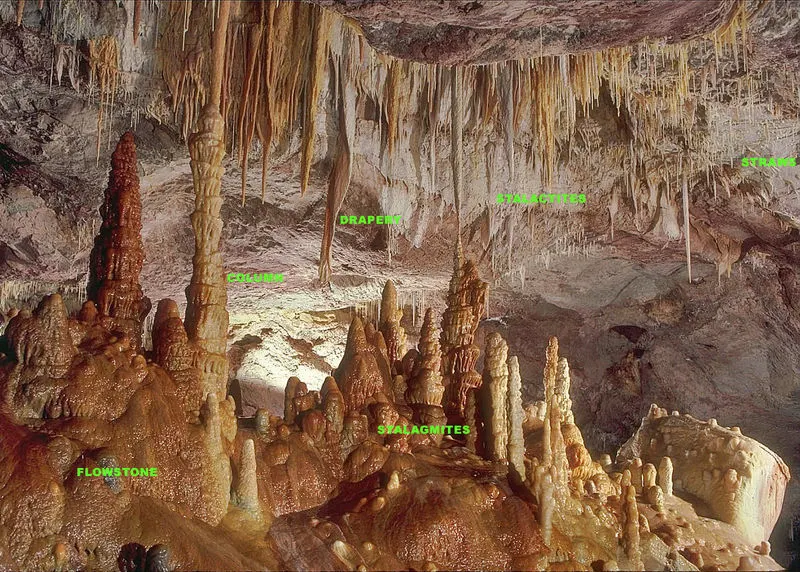
Fig 1.7:-stalagmite

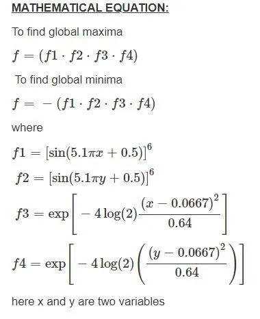
-Mathematical formula to calculate maxima and minima of stalagmite:-

code:-

%defining stalagmite function

function [f] = stalagmite_func(input_vector)
x = input_vector(1);
y = input_vector(2);



f1_x = (sin(5.1*pi*x+0.5)).^6
f1_y = (sin(5.1*pi*y+0.5)).^6
f2_x = exp(-4*log(2)*(((x-0.0667).^2)./(0.64)));
f2_y = exp(-4*log(2)*(((y-0.0667).^2)./(0.64)));

f = -1*(f1_x.*f1_y.*f2_x.*f2_y)
end

steps to execute the code:-

-we define output and input parameters of function and function name.

-we write a code to calculate input variables.

-for that, we use formula 0f global maxima and minima.

-we executed code to define our maxima and minima value of the stalagmite function.

code

-then we write our genetic algorithm code for statistical behaviour

close all
clear all
clc

%providing search space for the function

x = linspace(0,0.6,150);
y = linspace(0,0.6,150);
[xx, yy] = meshgrid(x,y);


%creating the surface plot of stalagmite function

for i=1:length(xx)
    for j=1:length(yy)
        input_vector(1)=xx(i,j);
        input_vector(2)=yy(i,j);
        f(i,j)=stalagmite_func(input_vector);
    end
end
surfc(xx,yy,f);
shading interp

Result:-

fval =

-0.0444

plot:-

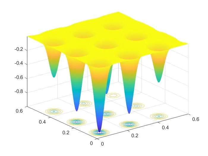
-steps that we followed to execute the code

1) first removing all residues of file with clear all,close all, and clc command

2) first we define search space for x and y with linspace command

3) then we created 2d mesh with the help of the mesh command

4) to create a surface of stalagmite function we executed for loop to run the code in between for loop for specific time

5) then we generated surface of stalagmite surface

6) then we call our stalagmite function which we assign to our ga inbuild function

7) then plot a graph of inputs vs stalagmite output f.

-after that, we tried out 3 studies to observe the statistical behaviour of a genetic algorithm

code:-

A) first study is to study no 1 stalagmite optimization to find global maxima for unbounded inputs:-

clear all 
close all
clc
%study no 1 stalagmite optimization to find global maxima for unbounded
%inputs
%defining the search space
x = linspace(0,0.6,150);
y = linspace(0,0.6,150);

%creating the 2d mesh
[xx,yy] = meshgrid(x,y);


%creating the surfacem plot of stalagmite function

for i = 1:length(xx);
    for j=1:length(yy);
        input_vector(1)=xx(i,j);
        input_vector(2)=yy(i,j);
        f(i,j)=stalagmite_func(input_vector);
    end
end

num_cases=50;  %ga runs for 50 num cases(iteration)
tic             %study time counter start

for i=1:num_cases
    [inputs, fopt(i)]=ga(@stalagmite_func,2);  %ga function is used to run the stalagmite data and give optimum solution
    xopt(i)=inputs(1);
    yopt(i)=inputs(2);
    
end


study_time=toc          %study time counter stops

subplot(2,1,1)
hold on
surfc(xx,yy,f)      %genrations of surface stalagmite function
shading interp      %to make smooth surface and remove grid lines
plot3(xopt,yopt,fopt,'marker','o','markersize',5,'markerfacecolor','r') %plotting the optimum value red dot mark along with 3d stalagmite curve
title('unbounded inputs')
subplot(2,1,2)
plot(fopt)          %plot fopt for every iterations
xlabel('num cases')
ylabel('function maximum')

Result:-

study_time =

149.5382\

Plot:- plotting num cases vs function maxima for unbounded inputs(num cases=50)

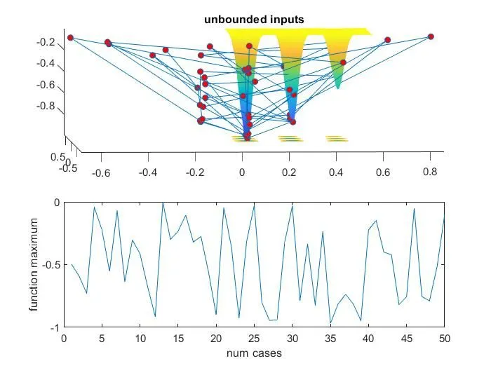
-in this study the bounds are not defined so the values of global maxima are going beyond of our boundary conditions.

steps that we followed to execute the code:-

1) first we remove all the residuals from script with clear all close all and clc command.

2) then we defined space for our inputs x and y with linspace command.

3) then we created 2d mesh with meshgrid command and executed for loop for 2d mesh of inputs xx and yy

4) then we took 50 num cases or u can say iterations and set a tic command to mark the starting time.

5) then we created a surface for stalagmite function for that we form a for a loop.

6) then created for loop for xopt ,yopt, and fopt

7) using ga function ga is used to run the stalagmite data and give an optimum solution.

8) after closing our for loop with the end command we mark the stop time.

9) then plot a subplot and generation of surface with a surface command of stalagmite function.
shading interp to make a smooth surface and remove grid lines.

10) then we plotted plot3 the optimum value red dot mark along with 3d stalagmite curve and define the title of the graph

11) then plotted a subplot and also fopt plot for every iterations.

12) the labeled our both axis.

code:-

B) the first study is to study no 1 stalagmite optimization to find global maxima for bounded inputs:-

clear all 
close all
clc
%defining the search space
x = linspace(0,0.6,150);
y = linspace(0,0.6,150);

%creating the 2d mesh

[xx,yy] = meshgrid(x,y);

for i = 1:length(xx);
    for j=1:length(yy);
        input_vector(1)=xx(i,j);
        input_vector(2)=yy(i,j);
        f(i,j)=stalagmite_func(input_vector);
    end
end
 num_cases=100    %ga runs for 100 num cases(iteration)
 tic              %study time counter start

 for i=1:num_cases
     %objective function is stalagmite and the number of variables are 2,
     %A,B.Aeq,Beq = [],as thair is no linear equalities and enequalities
     %constrain in this function
     %lower boundry in ga algo is set as [0;0]
     %upper boundry in ga algo is set as [1;1]
    [inputs, fopt(i)]=ga(@stalagmite_func,2,[],[],[],[],[0;0],[1;1])
    xopt(i)=inputs(1);
    yopt(i)=inputs(2);
    
 end
study_time=toc    % study time counter ends

subplot(2,1,1)
hold on
surfc(xx,yy,f)   %genrations of stalagmite function
shading interp   %to make smooth surface and remove grid lines
plot3(xopt,yopt,fopt,'marker','o','markersize',5,'markerfacecolor','r')%plotting the optimum value red dot mark along with 3d stalagmite curve
title('bounded inputs')
subplot(2,1,2)
plot(fopt)       %plot fopt for every iterations
xlabel('num cases')
ylabel('function maximum')

Result :-

study_time =

250.8188

Plot:- plotting num cases vs function maxima for bounded inputs.(num cases=100)

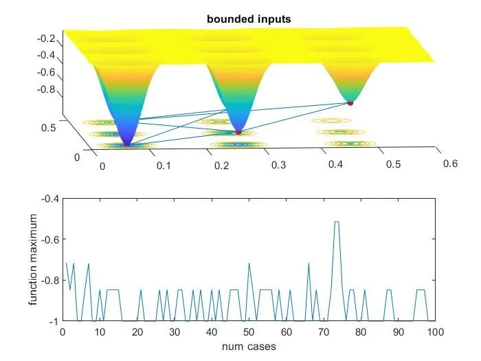
-in this study the plot is more clear and optimized value because the bounds were defined and we are getting values withing range.

-steps that we followed to execute the code:-

1) first we remove all the residuals from script with clear all close all and clc command.

2) we defined space for our inputs x and y with linspace command.

3) then we created 2d mesh with meshgrid command and executed for loop for 2d mesh of inputs xx and yy

4) the we took 100 num cases or u can say iterations and set a tic command to mark the starting time.

5) the we created surface for stalagmite function for that we form a for loop.

6) then created for loop for xopt ,yopt, and fopt

7) here syntax for ga function objective function is stalagmite and the number of variables is 2,
A,B.Aeq,Beq = [],as thair is no linear equalities and inequalities
constrain in this function
lower boundary in ga algo is set as [0;0]
upper boundary in ga algo is set as [1;1]

8) after closing our for loop with end command we mark the stop time.

9) then plot a subplot and generations of surface with the surface command of stalagmite function.
shading interp to make a smooth surface and remove gridlines.

10) then we plotted plot3 the optimum value red dot mark along with 3d stalagmite curve and define the title of the graph

11) then plotted a subplot and also fopt plot for every iteration.

12) the labeled our both axis.

CODE:-

C) the first study is to study no 1 stalagmite optimization to find global maxima for bounded inputs by increasing population size

clear all 
close all
clc
%defining the search space
x = linspace(0,0.6,150);
y = linspace(0,0.6,150);


%creating the 2d mesh
[xx,yy] = meshgrid(x,y);

for i = 1:length(xx);
    for j=1:length(yy);
        input_vector(1)=xx(i,j);
        input_vector(2)=yy(i,j);
        f(i,j)=stalagmite_func(input_vector);
    end
end
 num_cases=50     %ga runs for 50 num cases(iteration)
 options = optimoptions('ga')
 options = optimoptions(options,'populationsize',300) %expanding population size
 
  tic   %study time counter start

 for i=1:num_cases
     %objective function is stalagmite and the number of variables are 2,
     %A,B.Aeq,Beq = [],as thair is no linear equalities and enequalities
     %constrain in this function
     %lower boundry in ga algo is set as [0;0]
     %upper boundry in ga algo is set as [1;1]
     %population size is define is using by is in the algorithm
    [inputs, fopt(i)]=ga(@stalagmite_func,2,[],[],[],[],[0;0],[1;1],[],[],options)
    xopt(i)=inputs(1);
    yopt(i)=inputs(2);
    
 end
study_time=toc     % study time counter ends

subplot(2,1,1)
hold on
surfc(xx,yy,f)     %genrations of stalagmite function
shading interp      %to make smooth surface and remove grid lines
plot3(xopt,yopt,fopt,'marker','o','markersize',5,'markerfacecolor','r')%plotting the optimum value red dot mark along with 3d stalagmite curve
title('bounded inputs')
subplot(2,1,2)
plot(fopt)        %%plot fopt for every iterations
xlabel('num cases')
ylabel('function maximum')

Result:-

study_time =

430.1543

Plot:-plotting num cases vs function maxima for bounded inputs(num cases=50,population size=300)

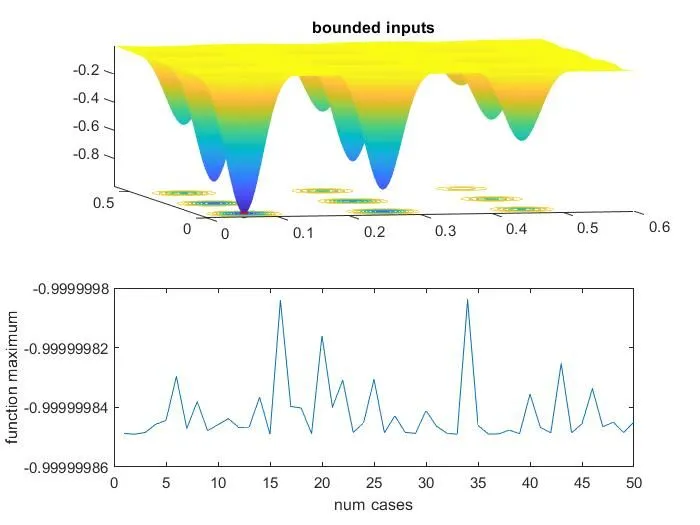
in this case, we are getting the optimum value of global maxima because we increase population size.

-steps that we followed to execute the code:-

1) first we remove all the residuals from script with clear all close all and clc command.

2) we defined space for our inputs x and y with linspace command.

3) then we created 2d mesh with meshgrid command and executed for loop for 2d mesh of inputs xx and yy

4) the we took 50 num cases or u can say iterations and set a tic command to mark the starting time.

5) also increase population size with help of optimizations.

6) then we created a surface for the stalagmite function for that we form a for loop.

7) then created for loop for xopt ,yopt, and fopt.

8)objective function is stalagmite and the number of variables is 2,

A,B.Aeq,Beq = [],as thair is no linear equalities and inequalities
constrain in this function
the lower boundary in ga algo is set as [0;0]
the upper boundary in ga algo is set as [1;1]
population size is defined is using by is in the algorithm

8) after closing our for loop with the end command we mark the stop time.

9) then plot a subplot and generation of the surface with a surface command of stalagmite function.
shading interp to make a smooth surface and remove gridlines.

10) then we plotted plot3 the optimum value red dot mark along with 3d stalagmite curve and define the title of the graph

11) then plotted a subplot and also fopt plot for every iteration.

12) the labeled our both axis.

ERRORS:-

while plotting surface plot put our outputs in round brackets so it was throwing an error saying "Invalid expression. When calling a function or indexing a variable, use parentheses. Otherwise, check
for mismatched delimiters" because our output is a vector to resolve this we simply used right parentheses which are square brackets represent vactor or matrix.

(note:-error screenshot is attached below)

RESULT:-

1) in an unbounded case study the bounds are not defined so the values of global maxima are going beyond our boundary conditions.

2) in a bounded case study the plot is more clear and optimized value than the unbounded case because the bounds were defined and also we increase the num cases(iterations) that's why we are getting values within a range.

3)in this case we are getting optimum value of global maxima because we increase population size (iterations)and our inputs are bounded.

CONCLUSION:-

To get the optimize value of global maxima we need to bound our inputs , also increase the iterations and increase the population size.

REFERENCES:-

1)All the figures (fig no 1.1 to fig no 1.6)related to phases of the genetic algorithm are taken from:-https://towardsdatascience.com/introduction-to-genetic-algorithms-including-example-code-e396e98d8bf3

2) syntax of ga is taken from:https://in.mathworks.com/help/gads/ga.html

3) fig no 1.7 stalagmites is taken from:-https://en.wikipedia.org/wiki/Stalactite#/media/File:Labeled_speleothems.jpg

(Note:-All the related result and error screenshots are attached below)

Week 4 - Genetic Algorithm

Ship work like this
in your own course.

Talk to a career counsellor

Ship work like thisin your own course.

Talk to a career counsellor

Ship work like this
in your own course.