Week 7 State of charge estimation
Aim :-
1].Simulate the 3 test cases from harness dashboard and write a detailed report on the results
2].What is coulomb counting? Refer to the above model and explain how BMS implements coulomb counting for SOC estimation ?
Steps:
Open the Design and Test Li-ion Battery Management Algorithm document in file exchange. Download the zip files, then extract them to a folder that contains the files listed below.
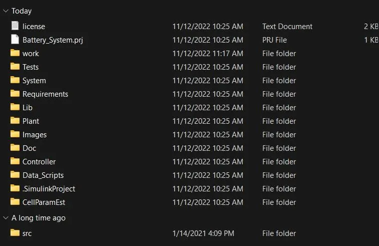
Open the closed loop BMS harness dashboard in tests simulink model file in Matlab. BMS Closed Loop Harness Model File for System. To install all the model-related library files into the current directories and workspace, give the dialogue box an open project and model.
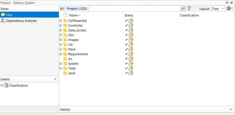
> Model file
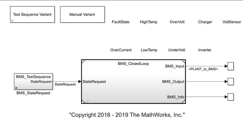
Model Explanation :-
1.DashBoard :-
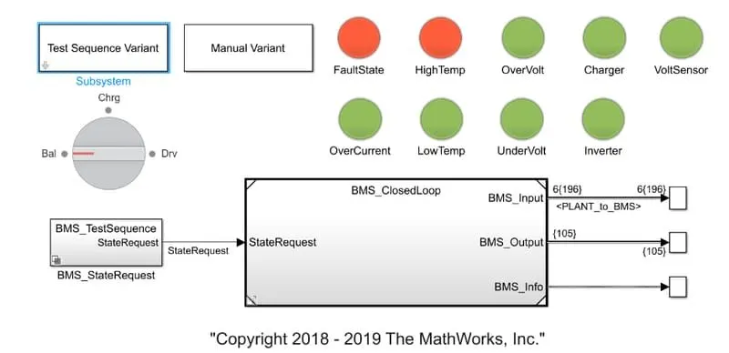
1. Test sequence varient.
2. Manual varient.
3. BMS_Test sequence state request to provide state request commands.
4.A faulty status, high temperature, over voltage, over current, charging voltage, sensor operation, inverter operation, low temperature, and under voltage are all shown by lamps. If there is a problem with any of these, a red indicator will let us know, and a green indicator will let us know that everything is well.
5.Rotating switch for manual varient changes while running simulation.
6. The module's SOC, module current, individual cell voltage, individual cell temperature, and battery condition are all considered outputs in the scope results.
2.BMS_Closed Loop :-
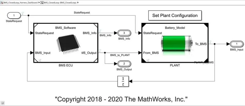
There are two subsystems—BMS ECU and PLANT units—in this main block. The plant output from the plant unit is provided as input to the BMS ECU as part of the BMS input feedback loop, and the BMS ECU unit receives the state request. The plant unit receives the state request from the BMS and the output commands as input.
BMS input, BMS output, and BMS info are the closed loop model's final outputs.
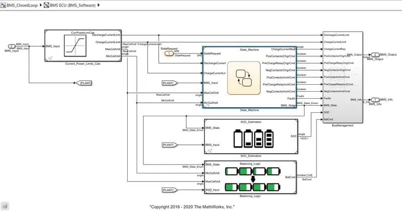
The calculations for the current power limit in the BMS ECU unit are carried out using the logics in the state machine block and Soc estimations cell balance as shown below.
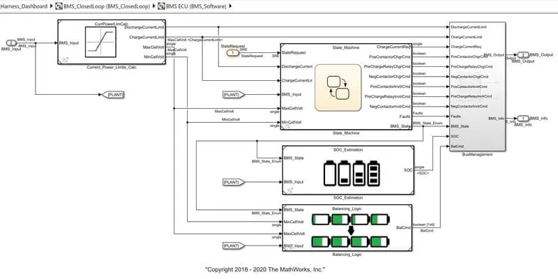
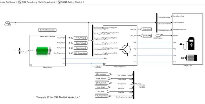
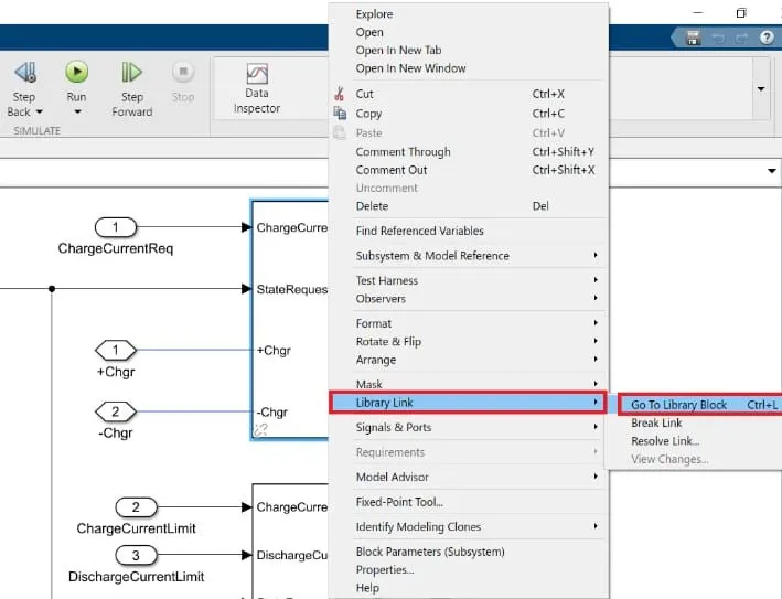
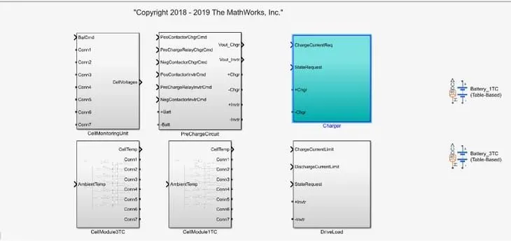
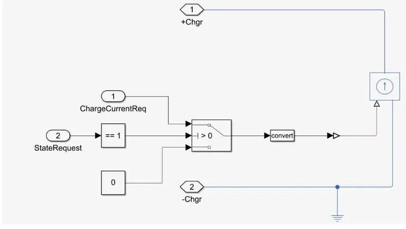
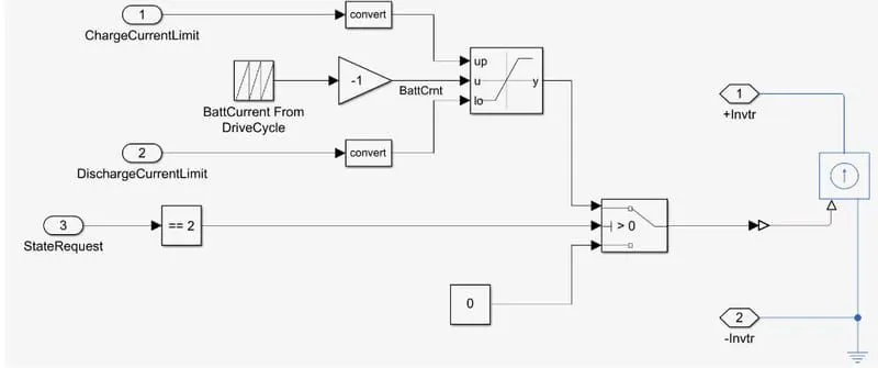
The battery pack unit, pre charge unit, charger, and load units are made in the plant unit.
The battery pack unit, pre charge unit, charger, and load units are made in the plant unit.
Here we are closing 1 module for lesser simulation running time.
1). To execute three test cases from the closed loop BMS control harness dashboard;
By choosing a test sequence variant and choosing the cases one at a time as follows, we must test three instances for this model.
case 1:
Select 1 from test sequence varient dialog box and click apply as shown below.
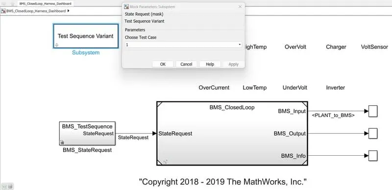
This selection includes such modifications to the masked BMS_State request system as,
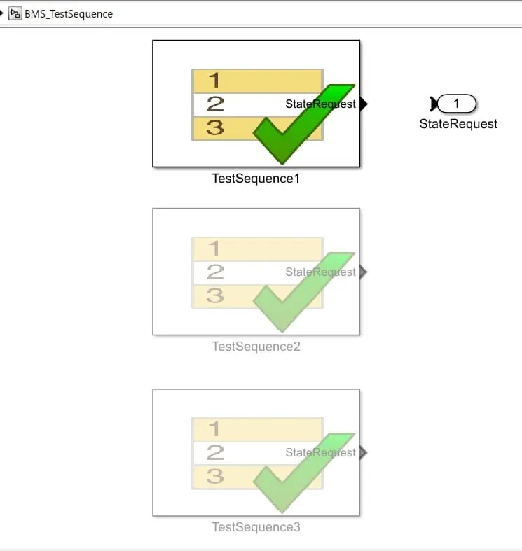
This test case consist of the following sequence operations,
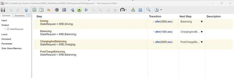
From the test sequence editor figure shown above, it was set as,
1. The first 3,000 seconds of driving.
2. Balancing operations start after 3000 sec and continue for the next 1000 secs.
3. The following 5000 seconds are spent on charging and balancing.
4. Following that, post-charge balancing operations continue until the simulation period is complete.
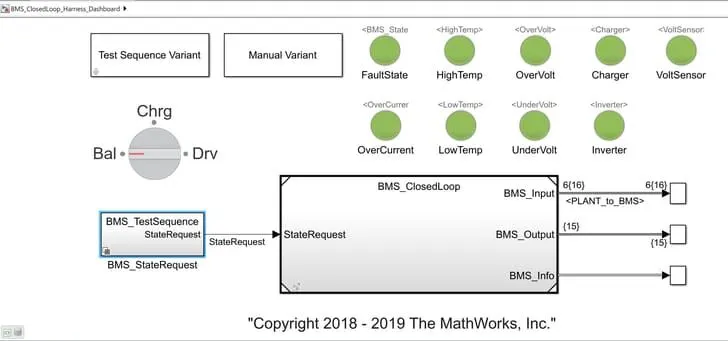
The model is fault-free because all of the lamp indications were green.
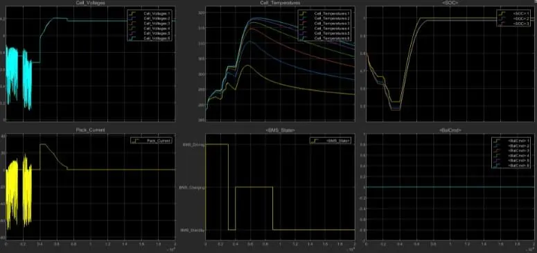
Results from running the simulation are shown as.
For the duration of the simulation, the lamp signals have been green, indicating that the procedure was flawless.
From the results, we may determine that,
Cell Voltage and Pack Current :
All 6 cells operate in drive mode for the first 3000 seconds, during which the majority of the discharging occurs, and standby mode for the last 1000 to 2000 seconds.
In this range, the voltage ranges from 3.1V to 3.9V. Cell balancing takes place between 3000 and 4000 seconds, during which time the module is in standby mode with a steady voltage of roughly 3.7V.
After 4000 seconds of charging, the voltage increased from 3.7V to 4V at 4.2V constant current as close to 30A, and then decreased from 4.2V constant voltage from 30A to 2.6A.
Cell balancing and charging take place for up to 9000 seconds. Post-charge cell balancing begins at 9000 seconds. According to the voltage shown with regard to cell 1, all cell voltages are balanced at 4.1V.
Cell Temperature :-
Cells' temperature range gradually rises from ambient temperature of 288 K to 302 K throughout the first 3000 s.
Cell has a lower temperature than cell 6, which is higher at all phases. After 4000 seconds, temperature begins to rise exponentially until the zone of constant current, and then it starts to fall as the current flow decreases in the region of constant voltage and cell balancing until 9000 seconds.
The maximum temperature in cells 1 and 6 was raised to 302 K and 317 K, respectively. The temperature continues to drop after 9000 seconds and stabilises at ambient temperature.
BMS State :
The battery module was in drive mode for 3000 seconds.
The battery module was in balancing standby mode from 3000 to 4000 s, as indicated.
The battery module is in charging and balancing mode from 4000 seconds up to 9000 seconds.
Only the post charge balancing mode functions after 9000 seconds until the simulation is finished.
SOC :
The battery module's initial state of charge is 80%. Here, the yellow curve represents a coulomb counting technique-based SOC estimation.
SOC estimate using the unscented kalman filter approach is represented by the blue plot. Extended Kalman Filter (EKF) and UKF provide more accurate estimates of SOC than coulomb counting approach, as shown in the red curve.
SOC initially drops to around 45% while in driving mode for the first 3000 seconds. Up to 4000 seconds later, the SOC remains constant at 45%, and cell balancing takes place in standby mode.
Module in charging mode from 4000 to 9000 seconds. As can be observed from the charts above, the SOC remained consistent after 9000 seconds at around 94%.
Balancing Cells :
Up to 3000 seconds, balancing did not take place. After 3000 seconds, cell balancing begins with cell 6 and cell 2, which have risen to the positions depicted. After this point, charging and balancing take place after charges have been balanced because cells 6 and 2 are still in a single state at the simulation's conclusion.
The cell stays in a 0 state throughout the simulation since it is operating at a lower voltage than the other cells. As we saw before in the signal cell votlage plot, all cell votlage attempts to balance evenly at the end of the experiment.
Case 2 :
Select Test Case 2 and then press Apply in the Test Sequence Variant dialogue box.
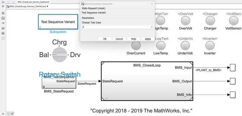
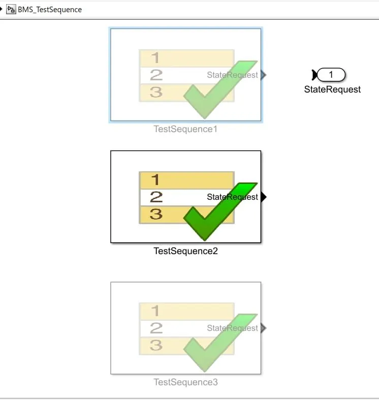
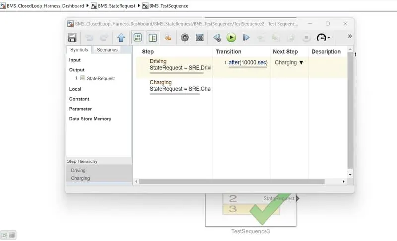
This test case consists of a drive mode for 10,000 seconds followed by charging that continues until the simulation is complete.
Scope result:
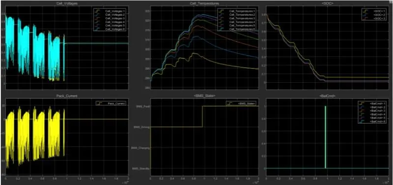
From the results, we may determine that,
Cell Voltage and Pack Current :
The cell voltage fluctuates from 3.9V to 3.05V as the cutoff voltage up to 9000sec, at which point the full capacity is used up. During the overall drive, the pack current discharges up to a maximum of 70A and barely recharges.
Conditions in the stand-by mode are in between those in the driving mode.
Cell Temperature :
The temperature in cell 1 in this example varied less, from 288 K to roughly 302.5 K. Temperature variation in cell number six ranges from 288 k to roughly 322.5 k. Since the cells are in standby mode between drives, the temperature of the cells is somewhat decreasing.
Battery Module State :
The entire sequence is running in drive mode, as indicated by the plot. A simulation command with a 10000sec duration is specified as the drive mode, therefore standby modes of shorter durations are not plotted in this plot.
However, standby modes are absent in actual practical situations, and other minor EVs consume battery power.
SOC of module :-
Here, the SOC decreased from 80% to 0% while the drive was operating. The SOC continues to be observable as seen in standby states in between them.
Balancing :-
Here, cell balancing is not done as indicated because the balance states are all zero during the driving mode.
Case 3 :
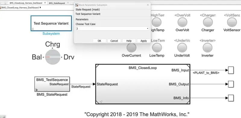
As illustrated below, pick Test Case 3 and then click Apply in the Test Sequence Varient dialogue box.
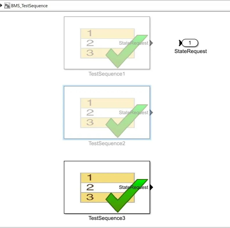
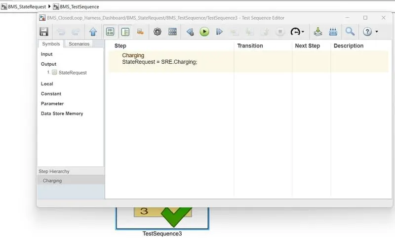
This test scenario includes charging for the full time.
Run the model and see the results,
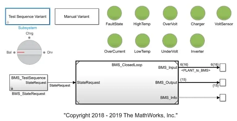
The model is fault-free because all of the lamp indications were green.
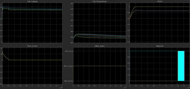
The plot resut shows that,
Cell voltage and pack current :
Cell 2's voltage initially increases from 3.9V to a maximum of 4.2V before stabilising at 4.15V. From 3.85V to 4.1V and then to 4.08V, Cell 1 increases.
The battery pack current increased from 0A to 30A before gradually decreasing to 2.5A at the conclusion of the 2000-second full charging cycle. Current flow will be stopped after a full charge, as seen in the result plot.
Cell Voltages and Pack Current :
The voltage in cell 2 initially increases from 3.9V to a maximum of 4.2V before stabilising at 4.15V.
From 3.85V to 4.1V and then to 4.08V, Cell 1 increases.
The battery pack current increases from 0A to 30A before gradually decreasing to 2.5A at the conclusion of a 2000-second complete charge.
The pack is 100% charged after 2000 seconds.
Current flow will be turned off following complete charge, as indicated by the result plot.
Cell Temperatures :
The cell temperature continues to rise until the battery is fully charged, at which point it begins to cool to room temperature.
As can be seen from the result plot, the temperature starts to drop after a complete charge.
BMS State :
The entire battery pack sequence is functioning as seen above in the charging mode.
SOC :
The pack SOC reaches full charge at 2000 seconds and maintains it for the remainder of the sequence as shown above.
By using UKF and EKF approaches, the true state of charge is approximately 93%, which is displayed as full charge.
Cell Balancing :
Here, starting at 0 seconds, cells 6 and 2 begin to balance with regard to cells 1 and all cells attempt to achieve balance at the conclusion of the simulation.
Thus, the performance of BMS on numerous parameters is examined and analysed using the aforementioned three test situations.
2) To explain coulomb counting for finding the SOC estimation in BMS;
Coulomb counting :-
SOC, which refers to the battery's remaining percentage, is defined as the rate of available capacity to its maximum capacity when a battery is fully charged.
We are utilising the coulomb counting approach to determine this SOC.
The battery's discharging current is measured using the coulomb counting method, which also integrates the discharging current over time to calculate SOC.
which can be calculated and estimated from the current being discharged and previously calculated SOC values,
SOC(t) = SOC(t - 1) + (I(t)/Qn)delta(t).
Modified Coulomb counting :
This method connects the discharge current to a function and calculates the corrected current to estimate SOC precisely.
Ic(t) = k2I(t)^2 + k1I(t) + k0,
where k0,k1,k2 are constant values obtained from the practice experimental data.
The SOC relation can be given,'
SOC(t) = SOC(t -1 ) + (Ic(t)/Qn)delta(t).
SOC estimation in BMS model :-
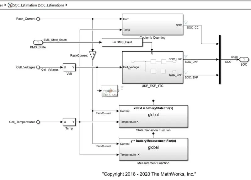
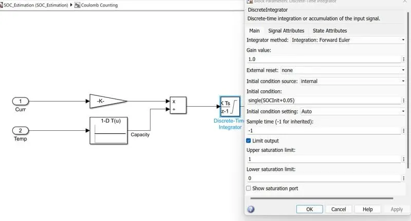
Click the SOC_estimation system's subsystem and select Coulomb counting to view the model for the coulomb counting technique in the BMS model.
SOC estimation in BMS model :-
Click the SOC estimation system's subsystem and select Coulomb counting to view the model for the coulomb counting technique in the BMS model.
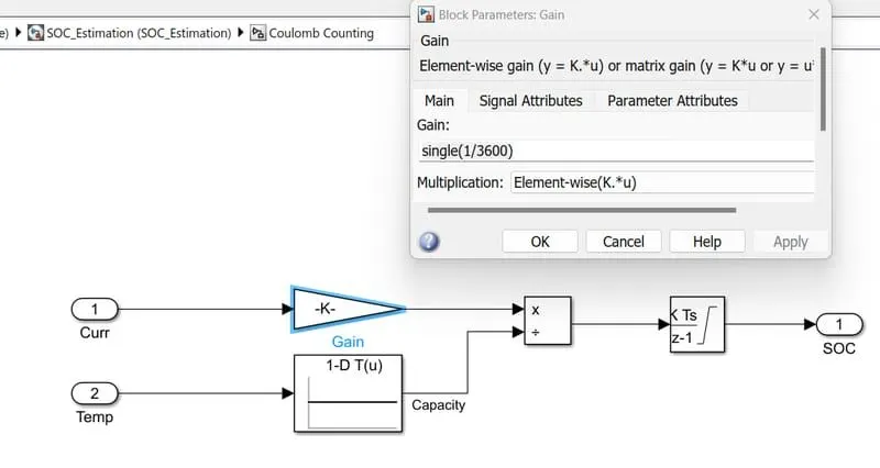
Here, the battery discharge current is converted to Ahr using a gain value of 1/3600.
As a result of temperature changes, the value is divided by the capacity. Then, since we are using a discrete integrator, we integrated with a gain value of 1 and sampling time 1.
We will multiply the SOC value, which ranges from 0 to 1, by 100 to obtain the SOC percentage.
Conclusion :
Consider simulating the three test cases from the harness dashboard and then summarize the findings in a report. Make use of the aforementioned model to demonstrate how effectively and concisely BMS performs coulomb counting for SOC estimate.