Week 7 State of charge estimation

OBJECTIVE 1

Battery Management system

How to Open ?

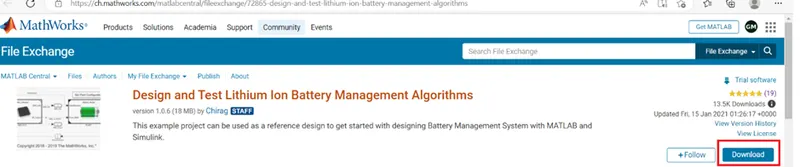
After Opening the below link, Click download for Battery Management system Zip file as shown in image

https://in.mathworks.com/matlabcentral/fileexchange/72865-design-and-test-lithium-ion-battery-management-algorithms

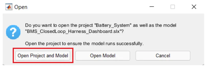
Go to Matlab open the Battery Model Project from saved folder as shown in image below

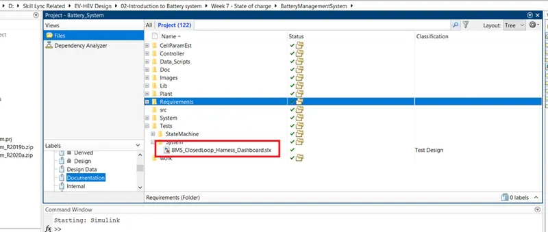
After this we have to open the Model from the Folder test as shown in image below

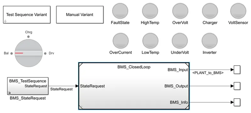
We will have model as shown in picture below

EXPLANATION OF TEST SEQUENCE SIMULINK MODEL

We have Test Sequence variant Block having 3 variants, each variant is ran for 3 modes Balancing mode, Charging Mode, Driving mode.

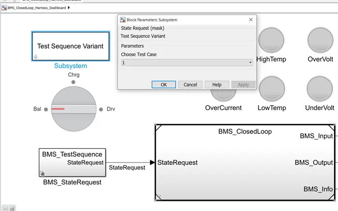
Select each variant and run the 3 test sequence.

TEST SEQUENCE 1:

Select the test sequence 1 as shown in image below

After selecting we can check in the BMS_Test sequence block as shown in image below

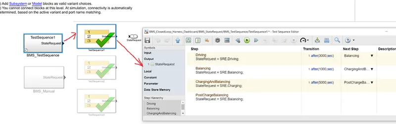
The above figure tell us about the test sequence running parameters:-

1. Driving Mode request is done for first 3000 sec.
2. Then balancing mode request of cell occurs for the next 1000 sec duration.
3. Then balancing Charging and balancing occur for next 5000sec
4. Post Charge Balancing is occurring after 9000sec till 20000 sec (i.e. simulation end time.)

Output Results:-

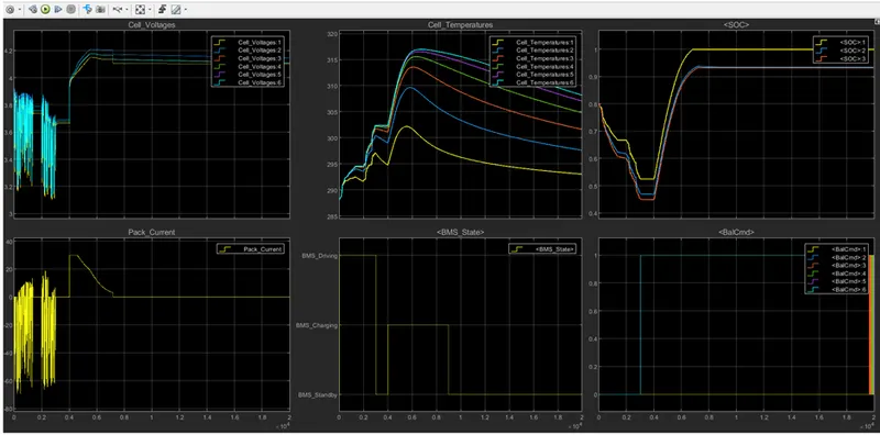
1) Driving mode (0-3000 secs):

• For the first 3000 secs are in driving state so the discharge of all the cells occurs and its varies in the range of 3.1 V min. to 3.9 V max.
• Cell temperature increases from 288K to 302 K.
• SOC also reduces from 80 % to 45%.

2) Balancing mode (3000-4000 secs):

• After 3000sec for 1000 secs, cell balancing occur and the Modules are in standby mode and they are having constant voltage near about 3.7V.
• Cell temperature reduces slowly as no current flow through the cells during balancing.
• SOC is also constant during this period at 45% .

3) Charging and Balancing mode (4000- 9000 sec):

• After 4000 sec the charging occurs and the cell voltages increased from 3.7 to nearly about 4.2 V in Constant current mode with current of nearly 30A and then the constant voltage charging starts and current reduces from 30A to 2.5 A Charging and balancing of cells occur till 9000 sec.
• Cell temperature also start to increase exponentially up to constant current region and reduces as current flow reduces in constant voltage mode.
• SOC also increases from 45% to 94%.

4) Post charge Balancing mode (9000- 20000sec):

• After 9000 sec the post cell balancing starts under standby mode.
• Cell temperature reduces in this mode and tries to reach the ambient temperature.
• SOC remains constant to 94%.

TEST SEQUENCE 2:

Select the test sequence 2 as shown in image below

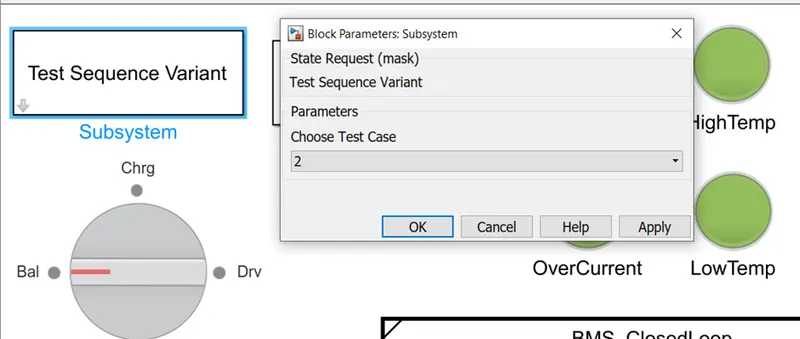
After selecting we can check in the BMS_Test sequence block as shown in image below

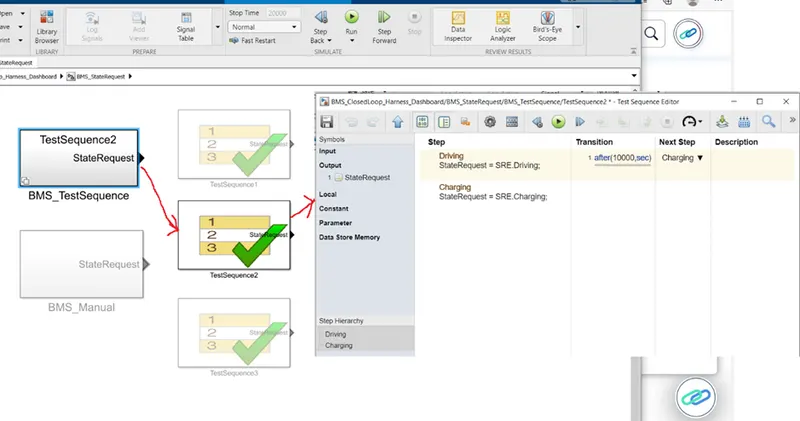
The above figure tell us about the test sequence running parameters:-

• Driving Mode request is done for first 10000 sec.
• Then charging mode done for next 10000sec.

Output Results:-

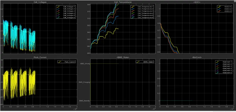
1) Driving Mode (0-10000 sec):-

• The cell voltage varies from 3.9 V to 3.05 volt which is cut off voltage of cell and the entire cell is drained up to approx. 8600 sec.
• Cell temperatures varies from 288K to approx. 320K.
• SOC reduces from 80% to 0% (cell got fully drained) in the drive mode under approx. 8600 sec.

2) Charging Mode (10000- 20000 sec):

• The cell got drained earlier before reaching this mode.

TEST SEQUENCE 3:

Select the test sequence 2 as shown in image below

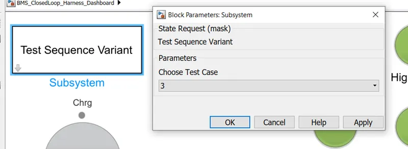
After selecting we can check in the BMS_Test sequence block as shown in image below

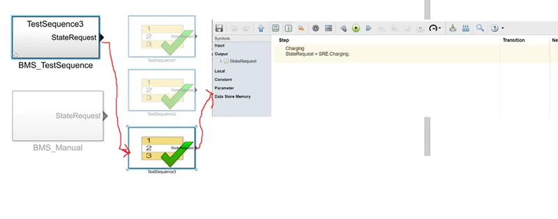
The above figure tell us about the test sequence running parameters:-

Charging mode done for entire simulation period 0 sec to 20000 sec.

Output Results:-

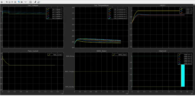
Driving Mode (0-20000 sec):-

• Cell Voltages increases from their initial values and after 2000 sec they got constant.
• Cell temperature starts to increases initially and when battery got fully charged then decrease down to the normal temperature.
• SOC was initially 80% and in 2000 sec it got fully charged that is 100%.
• Pack current initially start from 0 to 30A and then start decreasing when the constant voltage mode is there to 2.5 A up to 2000 sec then it is constant after full charge.

OBJECTIVE 2

State of Charge (SOC)

SOC of a cell or a battery at a given instant is the ratio of the charge available at that point to the charge available when it is full charged. It is expressed in percent, from 100% when full to 0% when empty. Analogous to how much fuel is available in cars tank.

Importance of SOC

• SOC indicates whether available charge is sufficient enough to carry out a particular function or not.
• Knowledge of SOC helps in operating the battery in the limits of charge and discharge.
• Very high or low SOC tends to permanently damage to battery.

SOC estimation is difficult as it represents internal state of the battery. There is no sensor /instrument to measure SOC directly. It needs to be inferred from battery voltage or battery current. Hence, the word SOC Estimation and not SOC measurement.

Some of the SOC Techniques shown in Table

Techniques	Advantages	Disadvantages
OCV	· Easy method · Useful to determine SOC at extreme ends.	· Long rest time required · Offline method · Not applicable to all battery types
Coulomb Counting	· Relatively easy computation · Online	· Accuracy affected due to drift · Sensor error cannot be rectified.
ANN	· Applicable to all battery types · Online · No battery mathematical model required	· Data driven model required · Huge data set for training the network
EIS	· Can be online · SOH information also available	· External instrumentation required
KF /EKF	· Online	· Large computational capacity required. · Battery model is required. · Works on assumptions
Fuzzy logic	· Online · Applicable to all battery chemistries.	· High computational cost.

We will discuss about Coulomb counting technique.

Coulomb Counting method:-

The coulomb counting method, also known as ampere hour counting and current integration, is the most common technique for calculating the SOC. This method employs battery current readings mathematically integrated over the usage period to calculate SOC values given by

where SOC(t0) is the initial SOC, Crated is the rated capacity, Ib is the battery current, and Iloss is the current consumed by the loss reactions.

The coulomb counting method then calculates the remaining capacity simply by accumulating the charge transferred in or out of the battery. The accuracy of this method resorts primarily to a precise measurement of the battery current and accurate estimation of the initial SOC. With a preknown capacity, which might be memorized or initially estimated by the operating conditions, the SOC of a battery can be calculated by integrating the charging and discharging currents over the operating periods. However, the releasable charge is always less than the stored charge in the charging and discharging cycle. In other words, there are losses during charging and discharging. These losses, in addition with the self discharging, cause accumulating errors. For more precise SOC estimation, these factors should be taken into account. In addition, the SOC should be recalibrated on a regular basis and the declination of the releasable capacity should be considered for more precise estimation.

Flowchart showing the algorithm

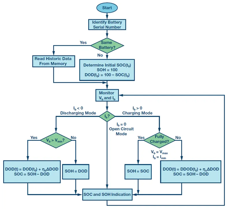
We will discuss the coulomb method in Test case Simulink model.

First open the BMS model as shown in image below

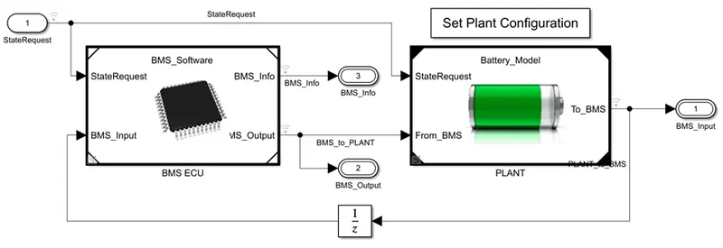
It has BMS ECU we have BMS software which the technique to find the SOC for the battery. In Plant model we will have a cells connected in series and parallel.

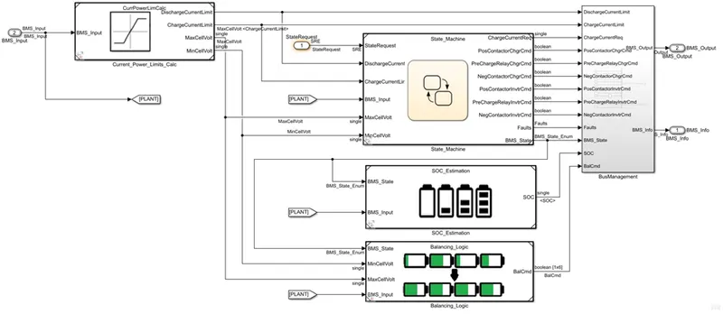
After opening the model we will have several models including SOC estimation model, image shows when we open it

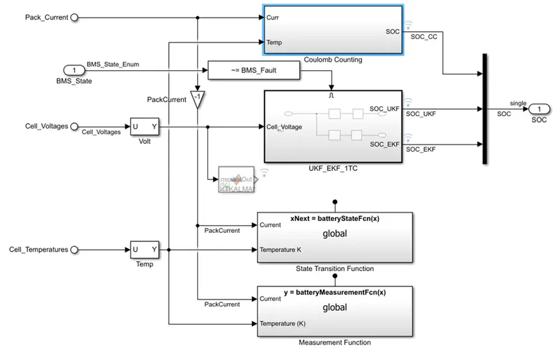
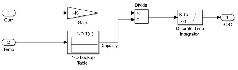
We have to open coulomb counting model to discuss

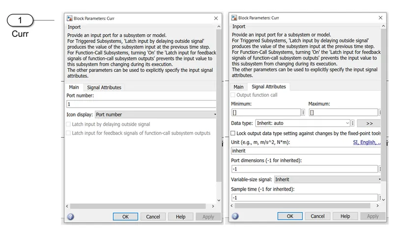
1) Input 1 - Current

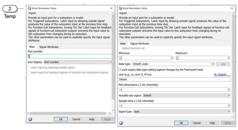
2) Temperature

3) Gain

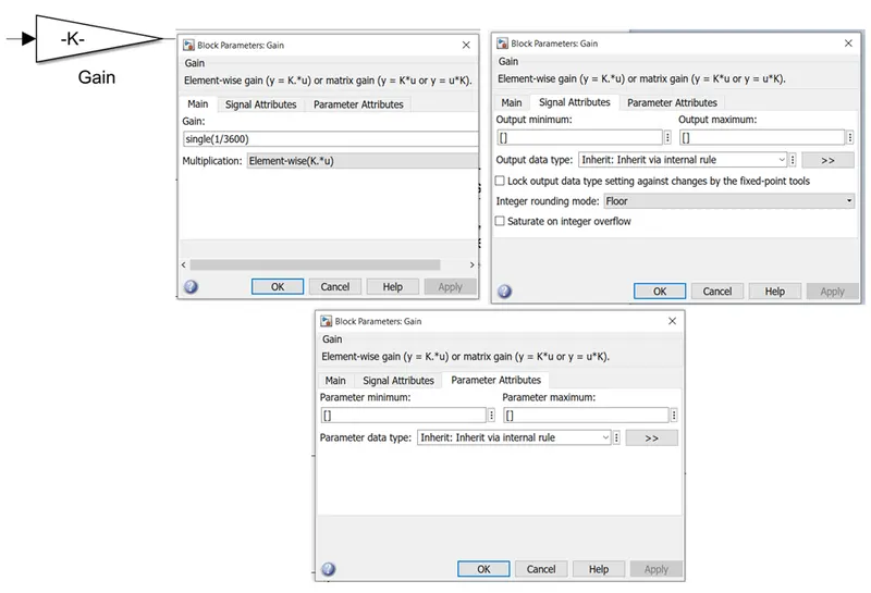
The Gain block multiplies the input by a constant value (gain). The input and the gain can each be a scalar, vector, or matrix.

Gain is converted from doubles to the data type specified in the block mask offline using round-to-nearest and saturation. The input and gain are then multiplied, and the result is converted to the output data type using the specified rounding and overflow mode.

4) 1D lookup model

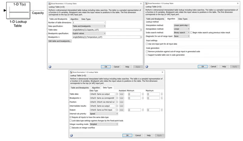
The 1-D, 2-D, and n-D Lookup Table blocks evaluate a sampled representation of a function in N variables.

5) Divide block

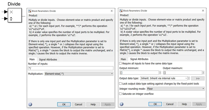
This block receives the input signal from the gain current and 1D look up temperature and then send the output to next block.

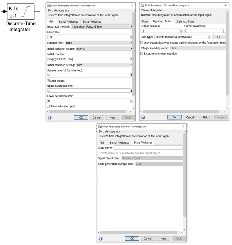
6) Discrete Time integrator Block

Use the Discrete-Time Integrator block in place of the Integrator block to create a purely discrete model. With the Discrete-Time Integrator block, you can:

• Define initial conditions on the block dialog box or as input to the block
• Define an input gain (K) value
• Output the block state
• Define upper and lower limits on the integral
• Reset the state with an additional reset input