Week 7 State of charge estimation
OBJECTIVE:
- Simulate the 3 test cases from the harness dashboard and write a detailed report on the results
- What is coulomb counting? Refer to the above model and explain how BMS implements coulomb counting for SOC estimation.
Hint :(Download the file from the link and go to SOC estimation model-ECU block)
OBJECTIVE-1:
- Simulate the 3 test cases from the harness dashboard and write a detailed report on the results
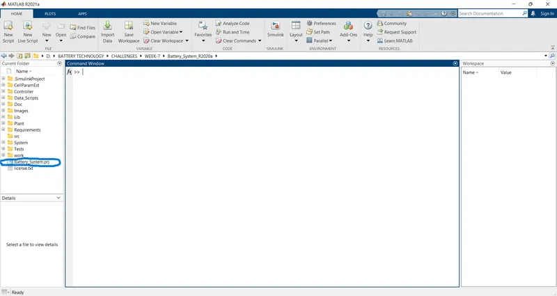
For this challenge, we have to download the reference file from the above-mentioned link. After downloading the zip format file extract the file into the folder. Then open MATLAB and select the file directory path where the reference file is saved folder. Then select the “Battery_System.prj” file to open the battery project file.
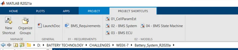
After opening the project file go to the project shortcuts tab then select the BMS SYSTEM.
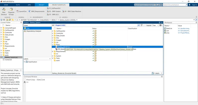
The new model will open then go to the Plant and select the Battery model simulation file and it will open in a new window.
Then go to the test>system> and select and open the battery closed loop harness file.
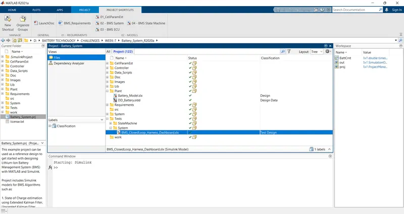
The three files are required to simulate the model. We simulate the model from the harness dashboard.
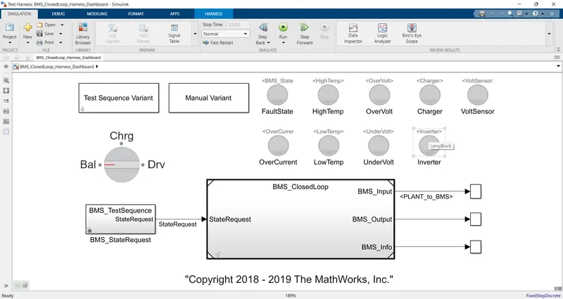
In the above figure, we can observe the different blocks and subsystems.
Blocks explanation:
Test Sequence Variant:
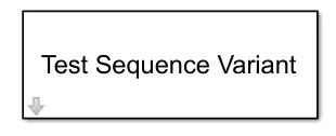
This block is used to select the various test cases. The above figure shows the test sequence variant block.
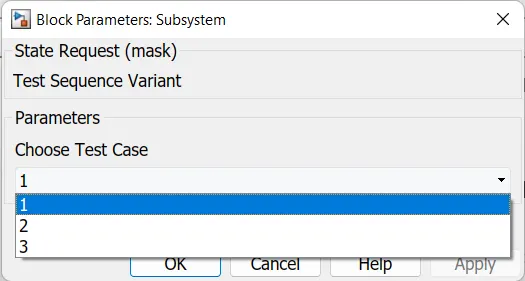
The test sequence variant block parameters are shown below.
Manual Variant:
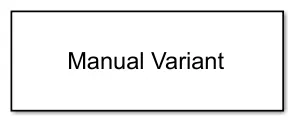
The above figure shows the manual variant block. By using this block we can simulate the model in the manual variant.
Rotary Switch:
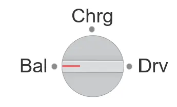
This rotary switch block has three terminals which are Bal, Chrg, and Drv. This block represents the conditions of the vehicle which is used in BMS.
The Bal terminal indicates the Balancing condition of the vehicle.
Chrg terminal indicates the Charging condition of the vehicle.
Drv This terminal indicates the vehicle is in driving condition.
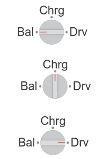
The above conditions are used in the manual variant simulation mode. When the simulation started the vehicle condition is changed by adjusting the rotary switch. Then we can observe the vehicle’s performance under various conditions.
In the below figure we can observe the rotary switch under various conditions.
BMS STATE REQUEST BLOCK:
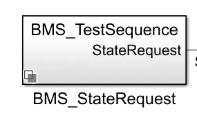
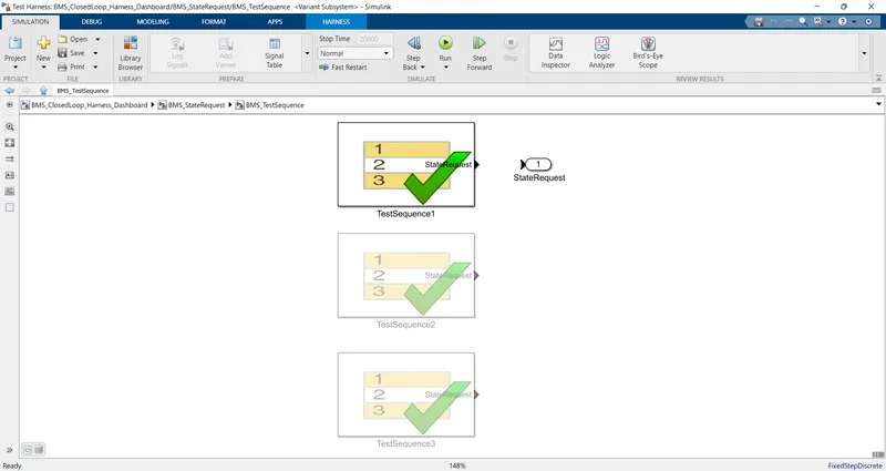
This block contains the test sequence conditions 1 to 3. It gives which test is to be performed if we set the case-1 then the state request will perform the first test and the other two tests are in off mode. The below figure shows the test condition-1 selection.
Lamp:
The lamp block diagram shows below.
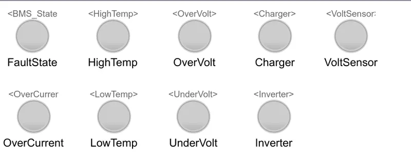
The lamp blocks which are attached to the dashboard will indicate if any fault happens. Any fault occurs lamps indicate in red colour. if no fault occurs all lamps indicate green colour.
TEST CASE -1:
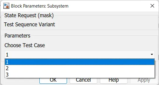
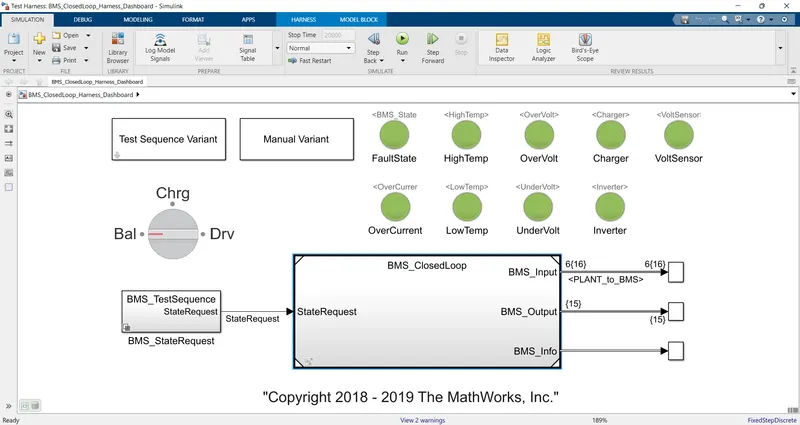
In this test case, we are taking the test sequence -1 and simulation the model for 20000seconds. All the lamps are indicated in green colour, so we can observe there is no fault occurred. Then we can change the test sequence to a manual variant and observe the Bal, Drv, and Charg modes of operation. The SOC, temperature of different cells, voltage, current, etc.
Plots:
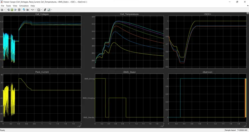
In the above plot, we can observe the voltage, current, SOC, temperature, BMS, state and Bal cmd.
Plot-1:
In the first plot, the initial stage to 3000seconds is in driving mode, so there are voltage fluctuations according to the driving conditions. The voltage varies from 3.2v to 3.8v. from 3000 to 4000seconds the vehicle is in a Balancing state, in this mode, the voltage of the cells settles at its nominal voltage of 3.7V. At 4000sec the voltage is in the increasing mode because after 4000seconds the mode will enter to charging and balancing state for 5000sec means till 9000sec, in this mode the cells get charged. So, it reaches its full charging voltage i.e., 4.2V and next it enters post-charge balancing mode where all the voltages get to settle to around 4.1V.
Plot-2:
In the second plot, we can observe temperature variations at each cell. From 0 to 3000sec is the driving mode, and the temperature of cells starts increasing according to the drive cycle. the balancing condition is from 3000 to 4000sec the temperature of the cells decreases gradually. After that charging and balancing mode will start from 4000 to 9000sec, where the temperature again starts increasing during charging and then starts decreasing for balancing mode. After that a slight decrement in the cell temperatures as it indicates the post-charge balancing mode.
Plot-3:
In this plot, the SOC changes according to the transition of the modes. In the driving mode, the SOC (state of charge) decreases from 80% to 45%. The SOC gets settled at 45%. After that charging and balancing mode will activate, where the cells get charged so the SOC will increases to 100% and then settles at full mode in post-charge balancing condition.
Plot-4:
In this plot we can observe the total pack, initially in the driving mode we can see the changes in current value according to the drive cycle. It varies from around -70A to 10A. When the vehicle enters into balancing mode then the current of the pack settles at zero. And when charging and balancing mode activates, the pack current will starts increasing it is around 30A and then gradually start decreasing to 0A. Later on, settles at 0A as the vehicle enters into post-charge balancing mode.
Plot-5:
This plot shows the BMS state. Like in which state the BMS is operating. We can see that on the y axis, three modes are pointed which are Driving, Charging and Standby. In driving mode i.e., till 3000sec the plot is at the driving point. After that for 1000sec i.e., till 4000sec, it will be in a standby position as it is in balancing mode. Then till 9000sec, it represents charging mode. Then it will settle at the standby position which represents the post-charging balancing mode.
Plot-6:
This plot shows balancing commands. Lie when the balancing mode activates then the plot reaches 1. So according to the balancing commands, the plots will settle.
Test Case-2:
From the test sequence variant, we are selecting test case-2. The below figure shows the test sequence block parameters.
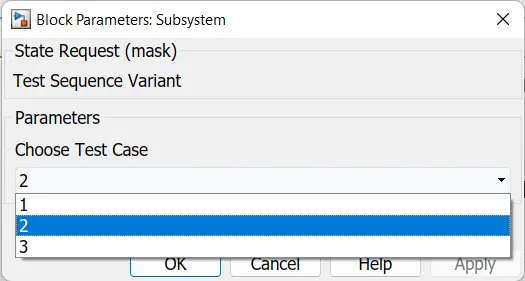
When the test sequence is changed to test case 2. In the BMS test sequence block, the state request is changed to two. And remain 1 and 3 are turned off.
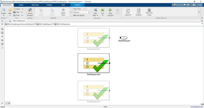
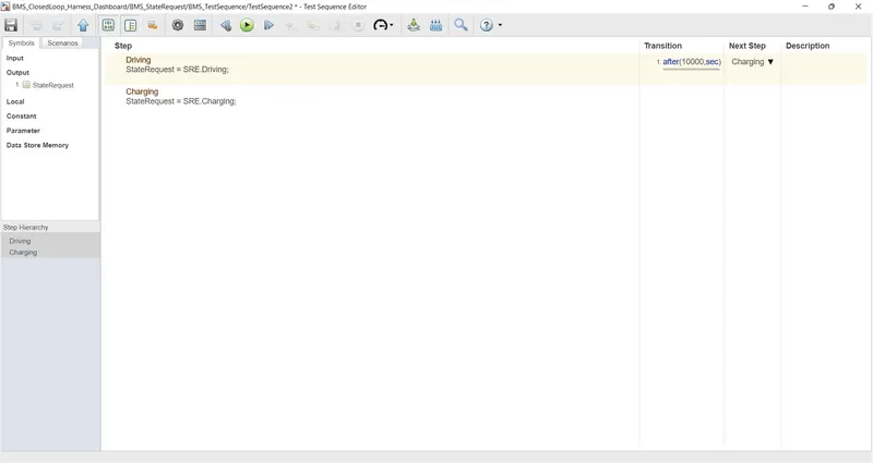
In this sequence, we can observe the two transitions. Initially, the driving condition will initiate for 10000seconds after this duration charging mode will activate.
After changing the test sequence simulate the model. After the simulation is completed we can observe the lamp’s indication.
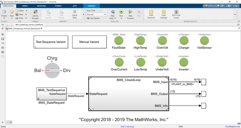
After the simulation, we can observe the results in scope. The following figure shows the scope block.
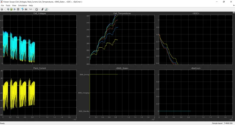
The result of test sequence-2 is shown in the above figure. In this simulation, only two modes Driving and Charging are activated and operated.
PLOT-1:
From the cell voltage plot, we can observe the voltage variation from 3.2V to 3.9V. this is the driving mode of operation. But due to the continuous driving, the voltage range is decreased from 3.1V to 3.7V.
PLOT-2:
In the second plot, we can see the temperature of the six cells. As the vehicle is in driving mode, the temperature is continuously increasing due to the high running time.
PLOT-3:
In the SOC plot, we can observe that the SOC is initially at 80% while driving the SOC starts discharging, even though there are charge and discharge conditions in the driving mode the running time is high so the SOC is reached its 0% at 8692seconds. So, it’s not even completed its driving duration also. Which we have set for 10000sec. So, all the plot stops at that time because at 0% SOC the vehicle stops then there are no other changes.
PLOT-4:
In the fourth plot, we can observe the current variations according to the drive cycle. Initially, it is varying between -70A to 15A. But with the long running time, the current value also comes to around -55A to 20A. And it ends after SOC reaches 0%.
PLOT-5:
In this plot, we can observe the BMS state of operation. Only the Driving mode is activated. So, the plot is maintaining a steady state in the graph.
PLOT-6:
In the last plot, we can see the Balcmd. Since there is no balancing mode it settles at 0 only.
Test Case -3:
For the third test case, we are choosing test sequence 3 in the test sequence variant. The test sequence block parameter is shown below.
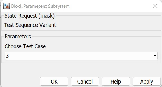
After changing the test sequence in the subsystem, the BMS state request third case is activated. And the remaining states are turned off. The below figure shows the test sequence3 selection.
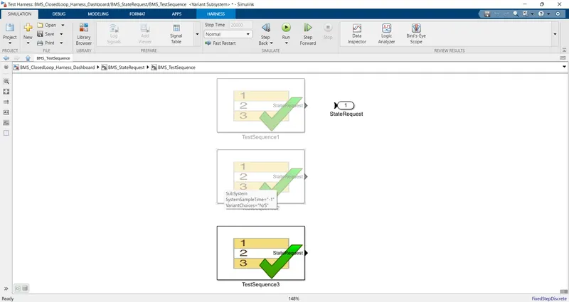
By opening the test sequence block we can observe that only the charge condition is present. So, the simulation is run in only charge mode.
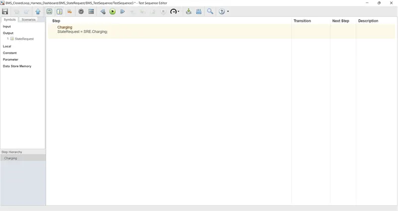
When the all changes are done and run the simulation. We can see the following dashboard.
The graph is plotted according to the test sequence operation.
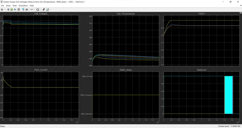
In this test sequence mode, only charge mode is activated and the remaining are turned off.
PLOT-1:
In this plot, we can observe the voltage reaches 4.2V, and then it will slightly decrease to 4.1V. this is charge mode only operated and maintains a 4.1V throughout the simulation. So, in this charge mode cell voltage has no variation.
PLOT-2:
From the temperature plot, it can be observed that while the battery is in charging condition there is an increment in the temperature of the cells. But after the battery is fully charged the temperature values are quietly settled at normal temperature.
PLOT-3:
In the SOC plot, we can observe that it is charged from 80% to 100% in 2000seconds and then it maintains its constant 100% throughout the simulation.
PLOT-4:
In the pack current plot, while the battery is in charging mode there is a rise in current from 0A to 20A, after the battery gets fully charged the pack currently comes to 0A and then settled.
PLOT-5:
This is a charging mode so the battery is only charged in this mode and no discharge happens. The BMS state plot shows only the charging.
PLOT-6:
As there is only a charging mode, the balancing mode maintains at 1. Which shows in the last plot.
OBJECTIVE-2:
- What is coulomb counting? Refer to the above model and explain how BMS implements coulomb counting for SOC estimation
What is coulomb counting?
The Coulomb counting method measures the discharging current of a battery and integrates the discharging current over time in order to estimate SOC. The coulomb counting method is done to estimate the SOC with respect to time. Which is estimated from the discharging current I(t), and previously estimated SOC values, SOC(t-1). SOC is calculated by the following equation.
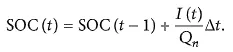
But there are several factors that affect the accuracy of the Coulomb counting method including temperature, battery history, discharge current, and life cycle. The coulomb counting method depends on the recording of the current noise only. The signal is filtered with a high pass filter with a cut-off frequency of 0.01Hz.
Modified Coulomb Counting method:
To improve the Coulomb counting method, a new technique called modified Coulomb counting method is proposed. The modified Coulomb counting method uses the corrected current to improve the accuracy of estimation.
The corrected current is the function of discharging current. There is a quadratic relationship between the corrected current and discharging current of battery. By practice of experimental data, corrected current is calculated by the following form:
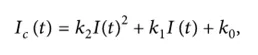
where , k2, k1 and k0 are constant values obtained from the practice experimental data.
In modified Coulomb counting method, SOC is calculated by the following equation:
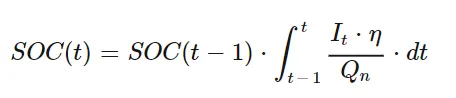
where,
SOC(t-1) = SOC at previous time step,
η = Efficiency,
t = Current time step,
Q = Charge capacity of the battery.
The experimental results show that the accuracy of the modified Coulomb counting method is superior to the conventional Coulomb counting method. The Coulomb counting method then calculates the remaining capacity simply by accumulating the charge transferred in or out of the battery.
How BMS implements coulomb counting for SOC estimation.
The BMS is implementing the coulomb counting for SOC estimation. The BMS system model block is shown below.
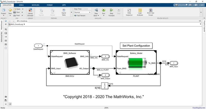
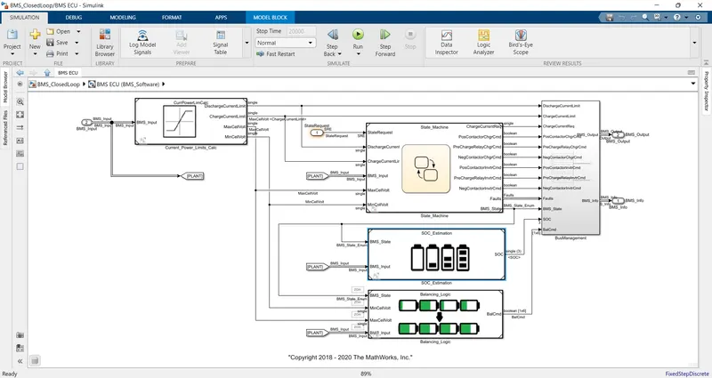
This model consists of the state machine, SOC estimation, and balancing logic subsystem. If we open the block SOC estimation we can find the coulomb counting subsystem.
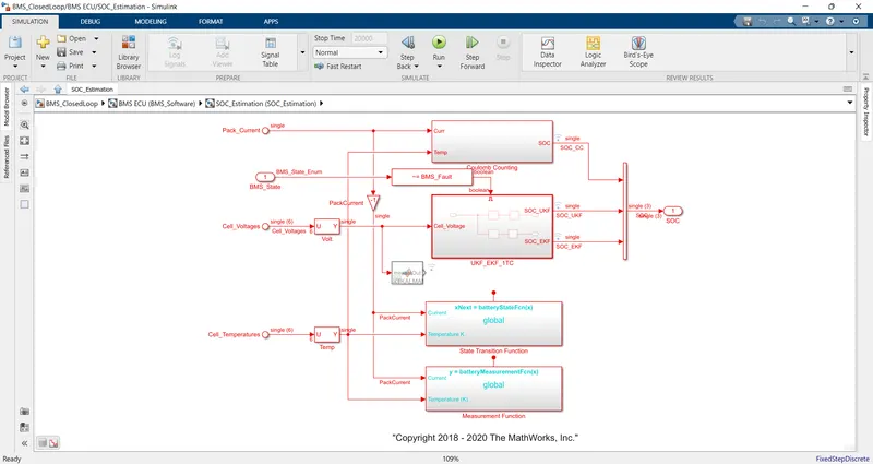
the coulomb counting subsystem block is shown below:
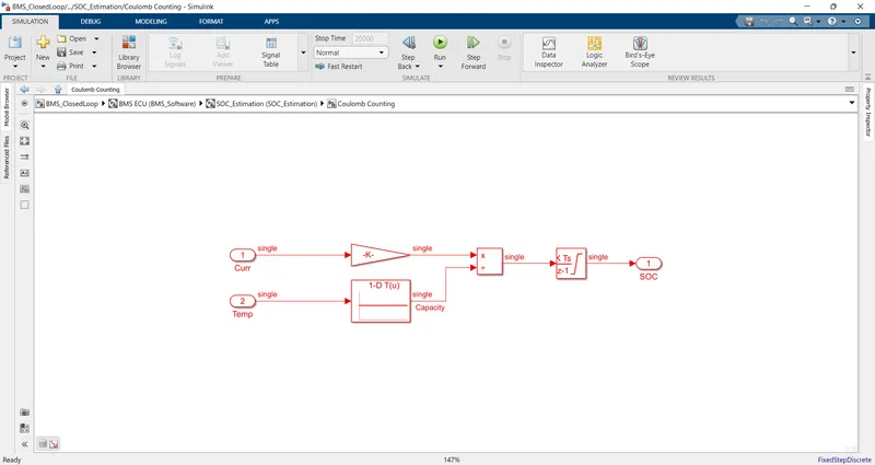
In the coulomb counting block, we can observe the different blocks. The current and temperatures are taken as input to gain block and lookup table block. The current is multiplied by the gain block and the output of the gain block is given to the product block.
The temperature is given to the lookup table and the capacity of the temperature is increased then it is given to the product block. By multiplying the temperature and current values then the output is given to the integrator block. The output of the integrator block is given to the outport of names as SOC. The main advantage of Coulomb counting is its simplicity, easy implementation, and low computational cost.