Week 7 State of charge estimation

Objective:

• The main objective of this challenge is to understand how the BMS (Battery Management System) will work and how to simulate the BMS model in Simulink, understanding the results obtained from the Simulink model.
• How to calculate the SOC (State of Charge) in Coulomb counting method and how BMS will implements Coulomb counting for SOC estimation.

Q-1: Simulate the 3 test cases from harness dashboard and write a detailed report on the results.

Model: (before running the test cases).

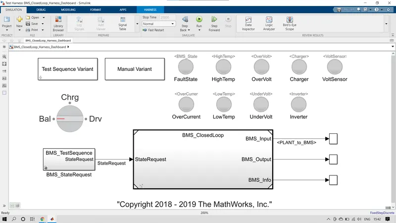
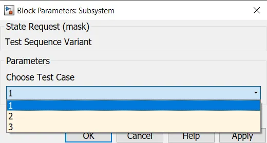
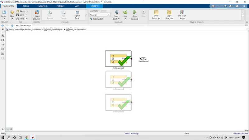
In the above given model, we need to give the test case number in the 'Test Sequence Variant' by double clicking on the sub-system. Once we selected the test case number in the Test Sequence Variant subsystem run the model, now the model will run 20000 seconds (time duration is default). When the simulation starts the output result graphs will open,

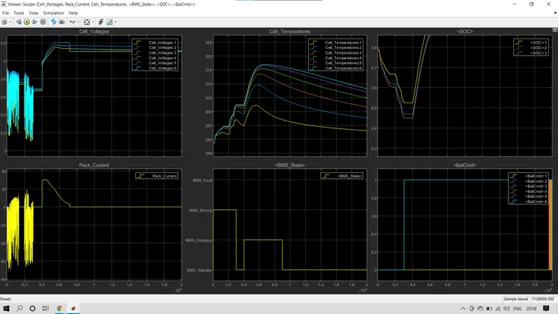
In the output results we can visualize 6 different graphs, those are

1. Cell voltage.
2. Cell temperature.
3. Cell temperature.
4. Pack current.
5. BMS (battery manageent syestem) state.
6. Balancing Command.

1stTest Case:

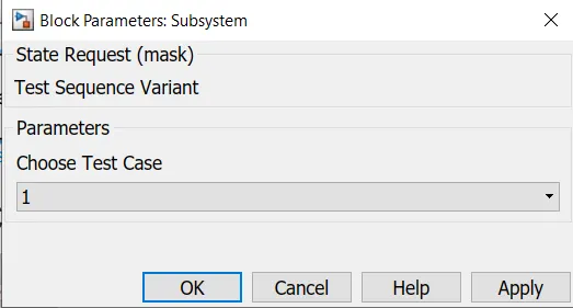
In the above given Test Sequence Variant, I selected the first test case to run the model. After running the model successfully we can visualize all the lamps will show's green colour to indicate, no errors occured while running the model. If the lamp shows red colour, the model has some problems while running it. Here in this case all the lamp blocks shows the green colour after finishing the simulation, that means there no problem in the model.

After simulation the dashboard and output graph are given below,

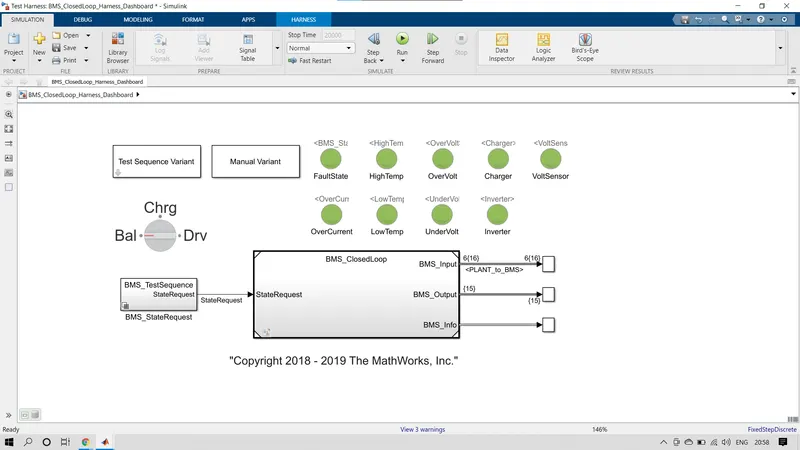
The above Dashboard model visualizes the first test case results with green colour in all the lamp blocks.

• The first graph ‘Cell voltage’ visualizes the cell voltage of all the cells in the entire battery pack, while simulating the model the cell voltages are changing as per the current flow (in and out). In the initial stage of simulation the, the voltages are slightly different because the model simulation was initialized with a slight associate of imbalance in the voltages are deflecting from 3.1V to 3.9V and the time period is 0.3*10^4 seconds. Now we can visualize the balance state of voltages their respective cells until the voltage of cells reach 4.2V, and it will remain till the end of simulation. We can observe a small voltage difference in their voltages and the voltage lies between 4V to 4.2V due the system is on standby mode.
• Now coming to cell Temperature, the temperature starts at 289 degrees and it will increases gradually, all the cells have different temperatures. The temperature traces shows the significant difference between the highest and lowest temperature cells, due to symmetry in the merged layers in terms of their thermal characteristics and behaviour. The 6th cell is high temperature cell and the 1st cell is lowest temperature cell due to it is thermally insulated at one side. In the graph we can visualize that the temperature of the cells will gradually increase till the time of 0.6*10^4 seconds and then the temperatures of all the cells will stars depleting gradually, at the end of the simulation the temperatures of all the cells are 293 degrees, 297 degrees, 302 degrees, 304.95 degrees, 307 degrees and 308 degrees.
• The SOC (state of charge) graph visualizes the differnt battery cell performances corresponding to coulomb count method, corresponding to ukf and ekf. The initial SOC is 75%, the starts at 80% to set their capability to recover. It is apparent that coulomb counting never does, because it has no way to get feedback to understand it is wrong due to its absence of voltage information. Both the algorithms recover on the other hand, from the initial error within the first hour of simulated time. With the ekf slightly outperforming than ukf.
• While in the charging state due to constant current phase, the current is lies between in the range of 19A to -70A in the time range of 0.3*10^4 seconds because maximum cell voltage is high. After 0.3*104^4 seconds the current will remain at 0A till 0.4*10^4 seconds and then the current will raise till the current attains 30A and the current will remains at 30A till 0.49*10^4 seconds. Now the current starts depleting gradually to around 2A and again it will depletes to 0A, from 0.7*10^4 seconds to till the end of simulation the current will remains at 0A.
• The other two scopes in result output visualizes the BMS (battery management system) and the balancing command signals respectvely.

2nd test case:

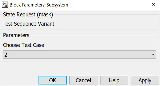
In the above given Test Sequence Variant, I selected the first test case to run the model. After the running the model successfully, in the dashboard we can visualize that the two lamp blocks will shows red color instead showing green color. That means, while running the test case two the simulationgone through some errors.

After simulation the dashboard and output graph are given below,

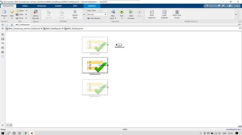
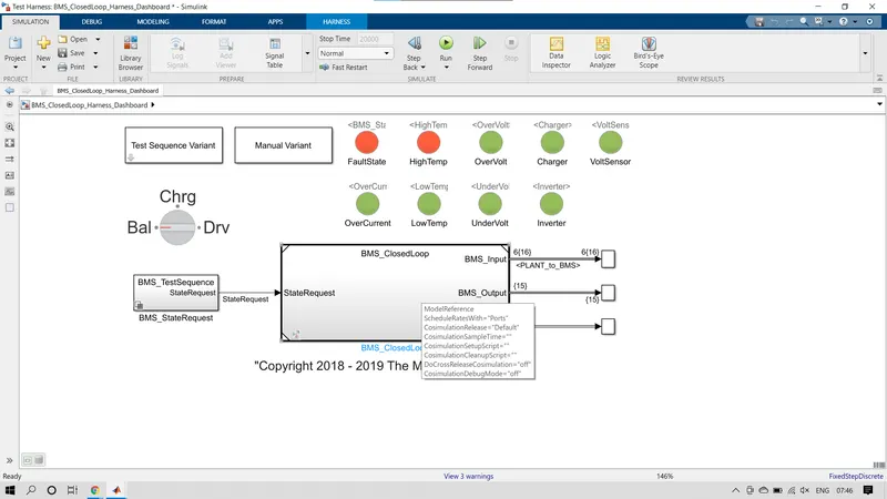
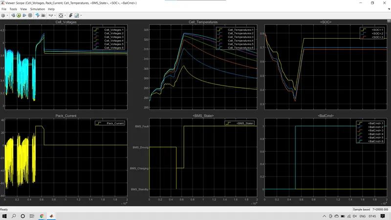
• The voltages of the cells in a battery pack will vary according to the current supplied to the cells. And the Voltages of the cells are lies between in the range of 3.18V to 3.9V till the time of around 1400 seconds and after 1400 seconds the voltage will be constant for each cells and the constant voltage line will remain till the 2000 seconds. After 0.2*10^4 seconds the voltage of cells will vary in the range of 3.1V to 3.85V up to the simulation time duration attains above 3800 second and after the voltages will remain constant, that constant voltage of individual cells will remain till above 4500 seconds and after the voltage will vary 3.1V to 3.75V and till 4500 seconds. After 4500 second the voltage will increase gradually to 4.1V till above 6200 second, after that the voltage will decreases to the 3.85V suddenly and the voltage will remains constant till the end of the simulation.
• The cell temperatures of the battery pack will be different for each individual cell. The cell number six has highest and cell number one has lowest temperatures. The cell one has a thermal insulation at one side, so the cell one temperature is low. The process initializes at 289 degrees and the temperature of the cells gradually increases till the simulation process attains above 6200 seconds and the temperature range is lies between 306 degrees to 323 degrees. After 6200 seconds the temperature graph starts depleting gradually till the end of the simulation. The temperature values are at the 20000 seconds for each cell are 294 degrees, 300 degrees, 304.5 degrees, 308 degrees, 311 degrees and 313 degrees.
• The state of charge for the cells initializes the simulation at 80% and the state of charge percent will deplete gradually till 4500 seconds and at 4500 seconds the state of charge is at 35%. After 4500 seconds the state of charge will starts increasing till SOC reaches to 69%, 70% and 76% until the simulation time attains above 6200 seconds and after the state of charge will remains same till the end of the simulation.
• The pack current will initializes the simulation process at 0A and the current will increase and decrease in the range between 10A to -70A and the current will be at 0A till the simulation attains 2000 seconds. After 2000 seconds the current will fluctuates up and down in the range between 9A to -65A till the simulation attains to 3900 seconds. After 4200 seconds the current will fluctuates 9A to -60A for 800 seconds and then the current will increases to 30A and it will remains for 1000 seconds. After 6000 seconds the current will depletes to 0A and the current will remains at 0A till the end of the simulation.
  The battery management system starts the process at BMS_standby state and it will moves to charging and driving state. The BMS is at driving state till 5000 seconds and after the BMS will goes back to standby state and than charging till 6200 seconds. After 6200 seconds the BMS shows BMS_fault indication due to lack of current and voltage. And the process will stuck at the BMS_fault till the end of the simulation.
• The balancing command graph visualizes that, the cell on will remains at 0 from initial state to end of the simulation. The cell six will starts at 0 and it will remains at 0 till 5000 seconds, after it will reaches to 1 and it will remains at 1 till the end of the simulation.
• The main reason to show the red flags on the lamp block in the dashboard is due to lack of current and voltage in the cells. With respect to current the voltage will vary, the temperature and SOC will vary with respect to the current and voltage. So the cell temperature reaches very high. Due to lack of voltage and current the BMS will shows the fault in the simulation process.

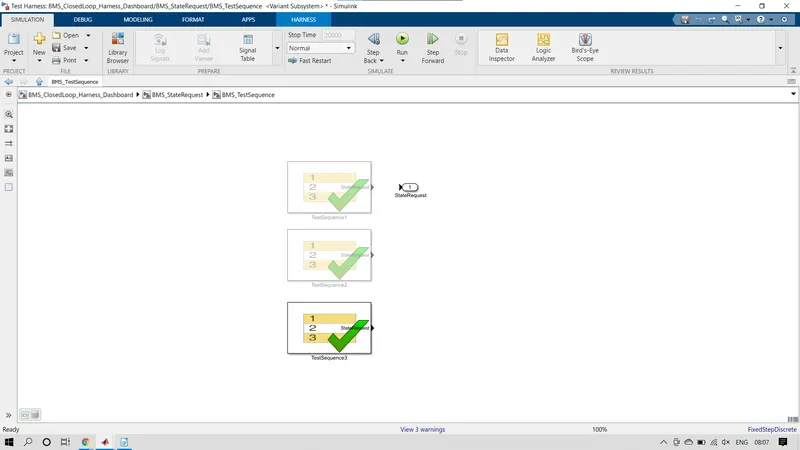
3rd Test case:

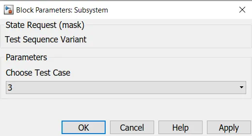
In the above given Test Sequence Variant, I selected the first test case to run the model. After the running the model successfully, in the dashboard all the lamp blocks shows green colour. That means while simulating the model the simulation process doesn't face any errors or difficulties.

After simulation the dashboard and output graph are given below,

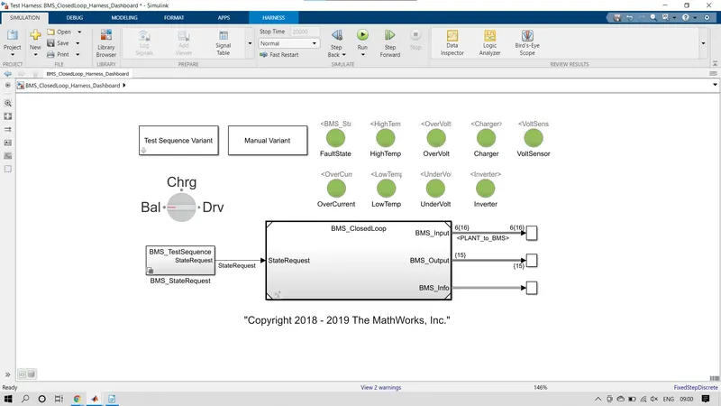
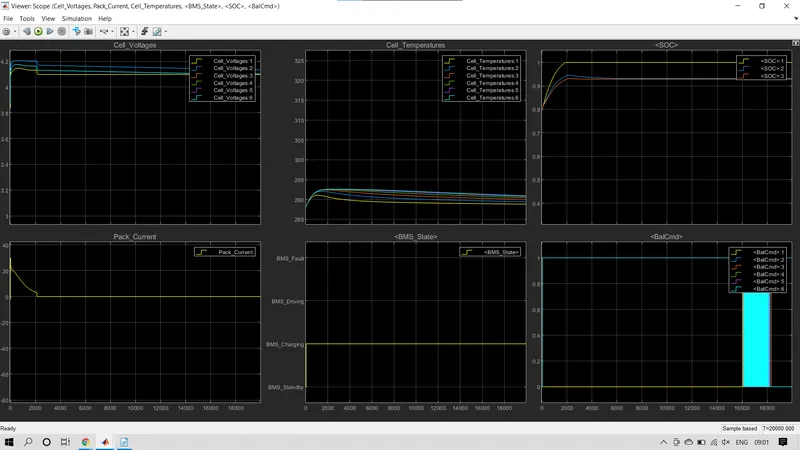
• All cells are initiated with different voltages, cell number six having higher voltage of 4.2V and cell number one having lower voltage of 4.1V and the remaining cells are falling under the range of BMS on charging state throughout the simulation and the voltage graph starts at 3.83V. Due to continuous voltage supply the graph is moving like a straight line, and we can visualize a very less amount of deflections in voltage of different cells. At the end of simulation the battery management system balances the voltage deflection in among the battery cells.
• The Cell Temperature graph starts at 288 degrees and the temperature will increase gradually till the time of around 1200 seconds and the maximum temperature at 1200 seconds is 293 degrees. And we can visualize the slight depletion in temperature till 0.4*10^4 seconds. After 4000 seconds the temperature is moves like a straight line, all the cells have different temperature ranges. The temperature traces shows the discrepancy in between the highest and lowest temperature cells, due to symmetry in the merged layer in terms of the cell thermal character and behaviour. Cell number six has highest temperature and cell number one has lowest temperature because the cell one has thermal insulation at one end. The active battery managements system will maintains a very less temperature difference between the cells.
• The State of charge for the cells starts at 80% and when the system under goes in a charging state, the yellow cell state of charge is will increase gradually to 100% and the remaining two cells are at 92% and 93%. The ukf and ekf initially having different charging rates, after 0.4*10^4 seconds the ukf and ekf are equal and the SOC is remains at 92% and the state of charge percentage is maintained through out the entire simulation. It is apparent that coulomb counting never does, because it has no way to get feedback to understand it is wrong due to its absence of voltage information. Both the algorithms recover on the other hand, from the initial error within the first hour of simulated time. With the ekf slightly outperforming than ukf.
• The battery pack current initialize the process at 20A and it depletes gradually 1A at the time range of 0.2*10^4 seconds. After 2000 seconds the current depletes to 0A, and it will remains at 0A till the end of simulation time.
• The other two scopes in result output visualizes the BMS (battery management system) and the balancing command signals respectvely. The Battery management system on charging state and Battery command passing signal between 0 to 1.

Q-2: What is coulomb counting? Refer to the above model and explain how BMS implements coulomb counting for SOC estimation ?

Coulomb counting is a technique used to track the state of charge of a battery pack. It works by integrating the active flowing current (measured in amps) over time to derive the total sum of energy entering or leaving the battery pack. This produces a capacity that is typically measured in Amph-hours.

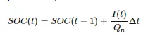
SOC(State Of Charge) is defined as the rate of available capacity to its maximum capacity when a battery is fully charged, and describes the remaining percentage of the battery capacity. To find this SOC % we are using coulomb counting method. The coulomb counting method measures the discharging current of the battery and integrates the discharging current over time in order to estimate SOC, which can be estimated from discharrging current(I(t)), previously estimated SOC values(SOC(t-1)).The relation is given below,

Modified coulomb counting method: In this technidue discharge current is corrected with a function and corrected current is found out for accurate SOC estimation. The function is given below,

here K0, K1 and K2 are constant values obtained from the practice experimental data. The SOC relation is given below,

The “coulomb counting” or CoulCount method was developed by Schmitt et al. as a heuristic method, although the underlying theory is reasonably accessible . It depends on the recording of the current noise only. The signal is filtered with a high-pass filter with a cut-off frequency of 0.01 Hz. The filter may be either analogue (although the implementation of a good-quality 0.01 Hz analogue filter is difficult) or digital. The absolute value of the measured current samples is then summed over time. A steep slope is taken as an indication of rapid corrosion, although it is not possible to calibrate this in terms of an estimated corrosion rate.

It can be shown that this method is similar to integrating the standard deviation of current over time. The use of the integrating plot provides a form of low-pass filtering that may make it easier to see trends, but this can also be accomplished by digital filtering. The use of only the current noise restricts the value of the technique, as it does not allow for the estimation of the noise resistance (and hence the corrosion rate), and it is difficult to see what real advantages the method has over the conventional three-electrode method, although the use of integrating plots may be of value.

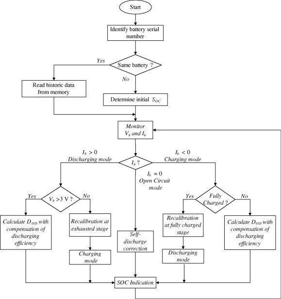
The flow chart to estimate the SOC state of charge is,

The SOC (state of charge) estimation model:

To see the SOC estimation model, we need open the different model block. The directions to open the SOC estimation modle is, BMS_ClosedLoop >> BMS ECU >>SOC_Estimation >> Coulomb Counting.

With the help of above mentioned directions, we can open the SOC estimation model and coulomb counting model.

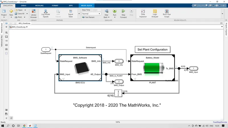
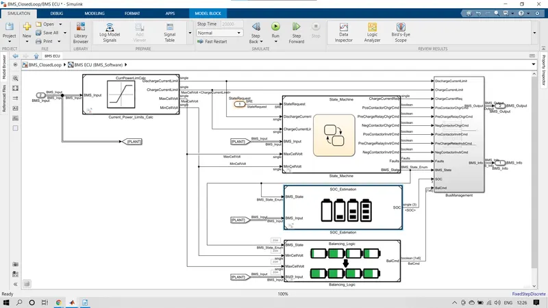
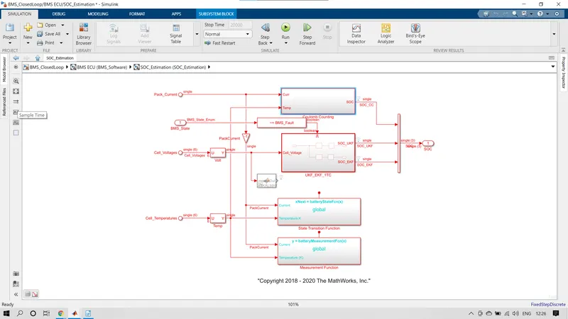
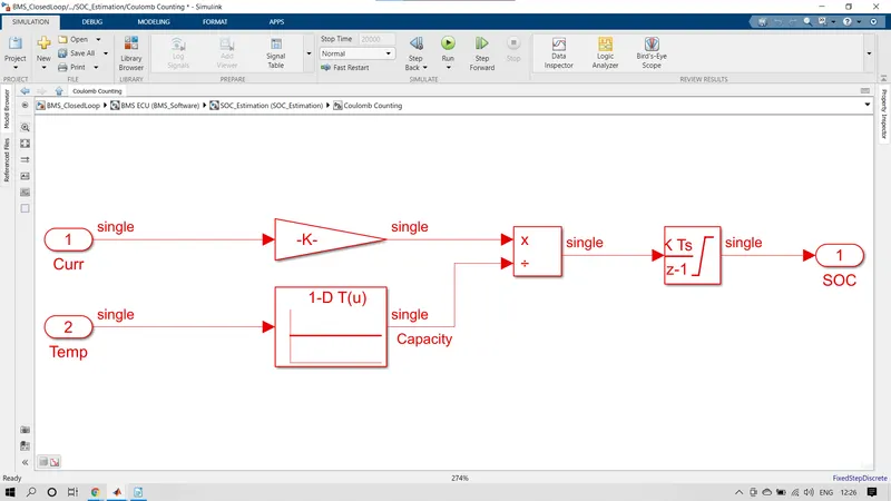
In the coulomb counting model, the pack current and temperature are the inputs for this model. The pack current is fed to the gain block with the vlue of 1/3600 to convert current in to Amph hours. The temperature is fed to the 1-D lookup table to give the inputs to divide block from the temperature input block. The Amph hour pack current and temperature get divided in the devide block and the output from the devide block is connceted to the Discrete- time integrator block to integrate the devided current and temperature signals.

From the output of discrete-time integrator block we can get the desired final SOC (state of charge). The block parameters of coulomb counting method are gioven blow,

• Input signals [Pack Current and Temperature (k)]:

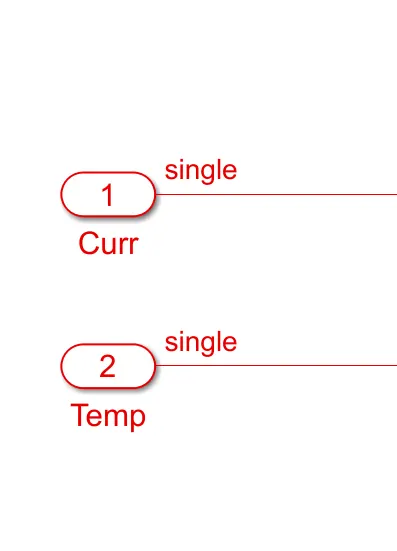
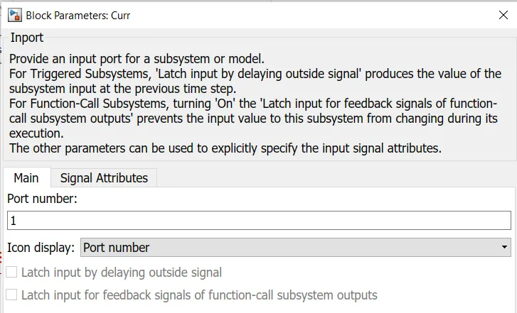
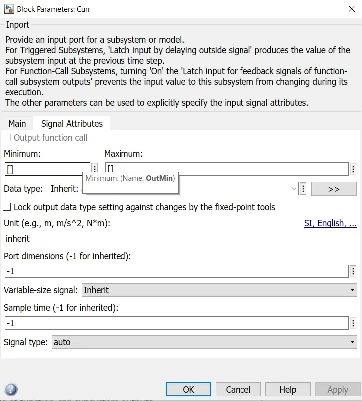
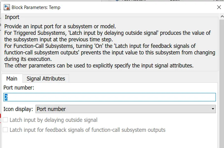
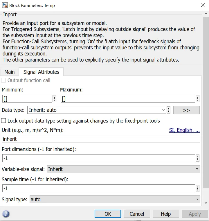
The input signals are fed to the coulomb counting model from other blocks in the project. the block parameters of pack current and temperature are

* Pack current:

* Temperature (k):

Gain block:

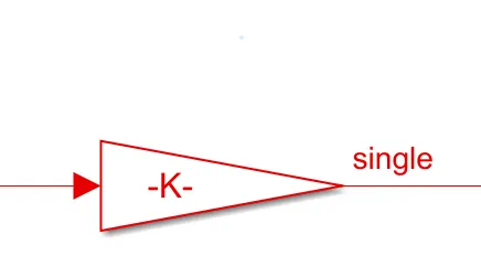
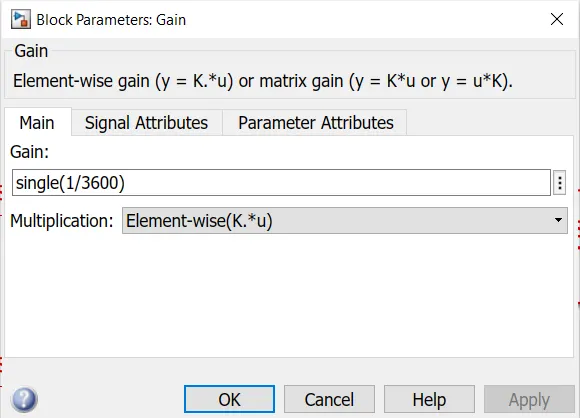
Here the discharge current from battery fed to the gain block with value of 1/3600 to convert current to 'Ahr'. The value is divided by capacity due to temperature change, then integrated with a gain value of 1 with sample time -1 as we are using discrete integrator. The saturation limits are from 0 to 1. We will get the SOC values from 0 to 1 multiplied with 100 to get in percentage of SOC.

• 1-D lookup table:

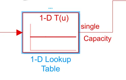
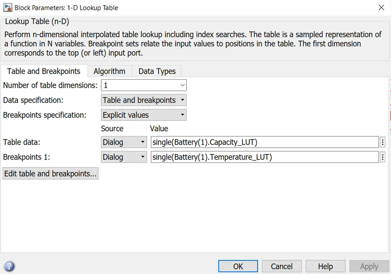
The 1-D lookup table is fed from the output of temperature input block. The lookup table is used to give the input to divide block.

Perform n-dimensional interpolated table lookup including index searches. The table is a sampled representation of a function in N variables. Breakpoint sets relate the input values to positions in the table. The first dimension corresponds to the top (or left) input port.

• Devide block:

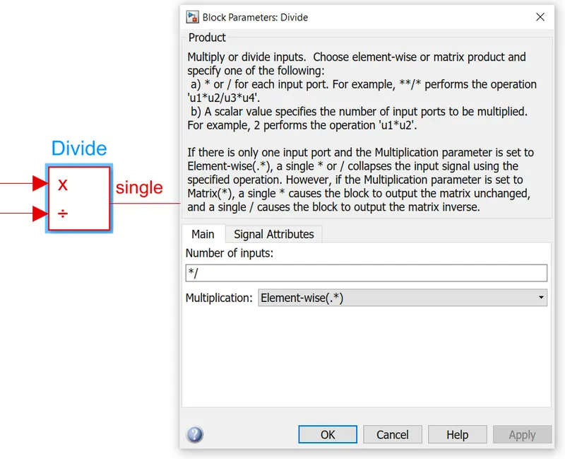
The divide block get the inputs from gain block pack current to multiply port and temperature from the 1-D lookup table to the divide port. the output from the divide block is fed to the discrete- time integrator block to integrate the divioded pack current and temperature signals to get the SOC.

• Discrete-time integrator block:

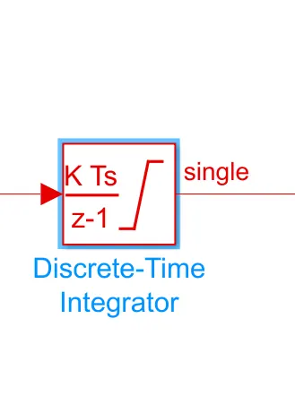
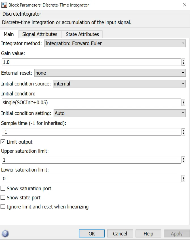
The integrator block get the inputs from the divide block. The devided pack current and temperature values are integrated in the discrete -time integrator to get the desired final SOC ( state of charge). The output SOC from the integrator block is fed to the output block to visualize the SOC in the results graph.