Week 3 - Solving second order ODEs

Aim: To solve `2nd` order ODE using MATLAB

Summary: 

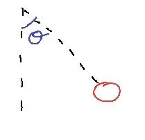
In Engineering, ODE is used to describe the transient behavior of a system. A simple example is a pendulum

Explanation:

The way the pendulum moves depends on the Newtons second law. When this law is written down, we get a second order Ordinary Differential Equation that describes the position of the "ball" w.r.t time. 

Similarly, there are hundreds of ODEs that describe key phenomena and if you have the ability to solve these equations then you will be able to simulate any of theses systems.

So we need to write a program that solves the following ODE. This ODE represents the equation of motion of a simple pendulum with damping

                         

                                                                                                                                                                       

In the above equation,

g = gravity in m/s2,

L = length of the pendulum in m,

m = mass of the ball in kg,

b = Damping coefficient

Using,

L=1 metre,

m=1 kg,

b=0.05.

g=9.81 m/s2

Motion = 0-20 secs

Angular displacement=0

Angular velocity=3 rad/sec

Time t=0

clear all
close all
clc

% Inputs
b=0.05;
g=9.81;
l=1;
m=1;

% Initial condition
theta_0 = [0;3];

% time points
t_span = linspace(0,20,100);

% solve ODE
[t, results] = ode45(@(t,theta) ode_func(theta, b,g,l,m),t_span, theta_0);

figure(1)
plot(t,results(:,1))
hold on
plot(t,results(:,2))
xlabel('Time')
ylabel('Plot')
legend('Angular Displacement','Angular Velocity')

% looping
ct=1;

for i = 1:length(results(:,1))
    
    x0 = 0;
    y0 = 0;
    
    x1 = l*sin(results(i,1));
    y1 = -l*cos(results(i,1));
    
    figure(2)
    plot([-1 1],[0 0],'linewidth',2,'color','k')
    hold on
    axis([-1.5 1.5 -1.5 1.5])
    plot([x0 x1],[y0 y1],x1,y1,'linewidth',2,'color','m')
    plot(x0,y0,'o','markersize',10,'markerfacecolor','g')
    plot(x1,y1,'marker','o','markersize',20,'markerfacecolor','y','markeredgecolor','b')
    pause(0.06)
    hold off
    M(ct) = getframe(gcf);
    ct = ct+1;
end

movie(M)
videofile = VideoWriter('Pendulum.avi','Uncompresssed AVI');
open(videofile)
writeVideo(videofile,M)
close(videofile)

function [dtheta_dt] = ode_func(theta,b,g,l,m)

    theta1 = theta(1)
    theta2 = theta(2)
    dtheta1_dt = theta2;
    dtheta2_dt = -(b/m)*theta2 - (g/l)*sin(theta1);
    dtheta_dt = [dtheta1_dt; dtheta2_dt];
end

In theta_0 = [0;3] ;

0 = Initial Displacement of the pendulum

3 = Initial Velocity of the pendulum

t_span = Time array; It goes from 0-20 secs with 100 values in-between

ode45 is an inbuilt solver

Output:

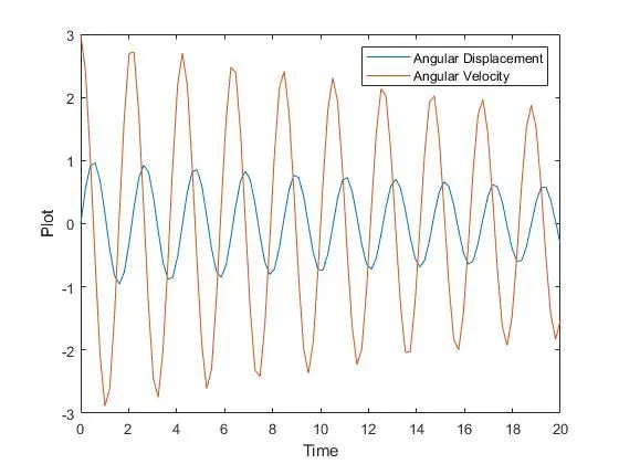
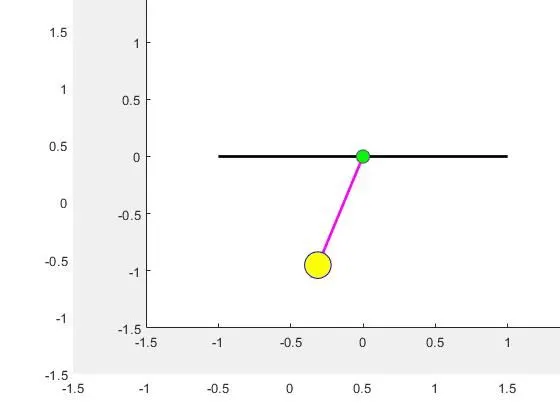
YouTube Link:

https://youtu.be/s9vy_qzOM2Q

Errors faced while programming:

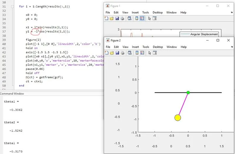
The pendulum was up-side down

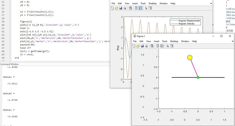
So, I had to assign "-" sign in line 37