Challenge

Week 4.1 - Genetic Algorithm

BBevan Christopher16 Feb 2022

Aim: To write a code in MATLAB to optimise the stalagmite function and find the global maxima of the function

Summary: In computer science and operations research, a genetic algorithm (GA) is a metaheuristic inspired by the process of natural selection that belongs to the larger class of evolutionary algorithms (EA).

Explanation:

GA:

Genetic algorithms are commonly used to generate high-quality solutions to optimization and search problems by relying on biologically inspired operators such as mutation, crossover and selection. Some examples of GA applications include optimizing decision trees for better performance, automatically solve sudoku puzzles, hyperparameter optimization etc

Syntax for ga:

x = ga(fun,nvars,A,b) finds a local minimum x to fun, subject to the linear inequalities A*x ≤ b. ga evaluates the matrix product A*x as if x is transposed (A*x').

example

x = ga(fun,nvars,A,b,Aeq,beq) finds a local minimum x to fun, subject to the linear equalities Aeq*x = beq and A*x ≤ b. (Set A=[] and b=[] if no linear inequalities exist.) ga evaluates the matrix product Aeq*x as if x is transposed (Aeq*x').

example

x = ga(fun,nvars,A,b,Aeq,beq,lb,ub) defines a set of lower and upper bounds on the design variables, x, so that a solution is found in the range lb ≤ x ≤ ub. (Set Aeq=[] and beq=[] if no linear equalities exist.)

example

x = ga(fun,nvars,A,b,Aeq,beq,lb,ub,nonlcon) subjects the minimization to the constraints defined in nonlcon. The function nonlcon accepts x and returns vectors C and Ceq, representing the nonlinear inequalities and equalities respectively. ga minimizes the fun such that C(x) ≤ 0 and Ceq(x) = 0. (Set lb=[] and ub=[] if no bounds exist.)

example

x = ga(fun,nvars,A,b,Aeq,beq,lb,ub,nonlcon,options) minimizes with the default optimization parameters replaced by values in options. (Set nonlcon=[] if no nonlinear constraints exist.) Create options using optimoptions.

example

x = ga(fun,nvars,A,b,Aeq,beq,lb,ub,nonlcon,intcon) or x = ga(fun,nvars,A,b,Aeq,beq,lb,ub,nonlcon,intcon,options) requires that the variables listed in intcon take integer values.

When there are integer constraints, ga does not accept nonlinear equality constraints, only nonlinear inequality constraints.

x = ga(problem) finds the minimum for problem, a structure described in problem.

example

[x,fval] = ga(___), for any previous input arguments, also returns fval, the value of the fitness function at x.

example

[x,fval,exitflag,output] = ga(___) also returns exitflag, an integer identifying the reason the algorithm terminated, and output, a structure that contains output from each generation and other information about the performance of the algorithm.

example

[x,fval,exitflag,output,population,scores] = ga(___) also returns a matrix population, whose rows are the final population, and a vector scores, the scores of the final population.

Stopping Criteria:

Stopping criteria determine what causes the algorithm to terminate. You can specify the following options:

MaxGenerations — Specifies the maximum number of iterations for the genetic algorithm to perform. The default is 100*numberOfVariables.
MaxTime — Specifies the maximum time in seconds the genetic algorithm runs before stopping, as measured by tic and toc. This limit is enforced after each iteration, so ga can exceed the limit when an iteration takes substantial time.
FitnessLimit — The algorithm stops if the best fitness value is less than or equal to the value of FitnessLimit. Does not apply to gamultiobj.
MaxStallGenerations — The algorithm stops if the average relative change in the best fitness function value over MaxStallGenerations is less than or equal to FunctionTolerance. (If the StallTest option is 'geometricWeighted', then the test is for a geometric weighted average relative change.) For a problem with nonlinear constraints, MaxStallGenerations applies to the subproblem (see Nonlinear Constraint Solver Algorithms).

For gamultiobj, if the geometric average of the relative change in the spread of the Pareto solutions over MaxStallGenerations is less than FunctionTolerance, and the final spread is smaller than the average spread over the last MaxStallGenerations, then the algorithm stops. The geometric average coefficient is ½. The spread is a measure of the movement of the Pareto front. See gamultiobj Algorithm.
MaxStallTime — The algorithm stops if there is no improvement in the best fitness value for an interval of time in seconds specified by MaxStallTime, as measured by tic and toc.
FunctionTolerance — The algorithm stops if the average relative change in the best fitness function value over MaxStallGenerations is less than or equal to FunctionTolerance. (If the StallTest option is 'geometricWeighted', then the test is for a geometric weighted average relative change.)

For gamultiobj, if the geometric average of the relative change in the spread of the Pareto solutions over MaxStallGenerations is less than FunctionTolerance, and the final spread is smaller than the average spread over the last MaxStallGenerations, then the algorithm stops. The geometric average coefficient is ½. The spread is a measure of the movement of the Pareto front.
ConstraintTolerance — The ConstraintTolerance is not used as stopping criterion. It is used to determine the feasibility with respect to nonlinear constraints. Also, max(sqrt(eps),ConstraintTolerance) determines feasibility with respect to linear constraints.

Study 1:

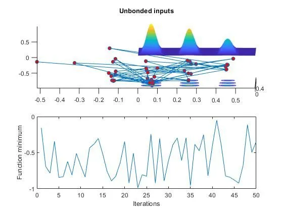
In case study 1 we will be just be applying the Genetic Algorithm and see how the program performs without any constraints.

So in the beginning we are providing the x and y inputs using the linspace command and the Num_Cases which is the iteration number. Since x and y are both a One-Dimensional array we are using the Mesh grid to form a Two-dimensional array represented by xx and yy.

This For loop will run for the length of the xx and yy, The input function is a row vector with two columns which we are assigning using Input_vector(1) and (2).

The Stalagmite function here will help us in finding the local maxima and minima. This loop is used entirely for the plotting of the 3-D Graph so that we can easily understand the working. The Stalagmite function is a function that we call into this program.

The Formula for the Stalagmite function is below:

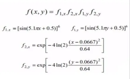
The two variables in the function are x and y. We need to convert this formula into Matlab code so that we can call it in.

We can see that F will be the output for the above function and, Input_vector(1) and Input_vector(2) being x and y. Then we code the formula as it is so that we find the value of F.

We already know that Ga will only find the Global minima (i.e) using the Stalagmite function it can only find the lowest value. So we need to make a small change in the final step of the function so that Ga will be able to find the Global maxima so we will be introducing a"-" sign to F so that Ga can find the Global maxima.

We will be creating two plots so we will be applying the subplot command. The surfc is used to view the 3-D graph of the points xx,yy,-F, Here the -F is to represent the graph in the positive axis. Hold on is used to views all the plots. Sharp interp is used so that the 3-D graph is more representable.

Plot 3 is used to plot all the three values xopt,yopt and -fopt in the 3-Graph and the second Subplot only views the fopt in a 2-D graph.

Study 2:

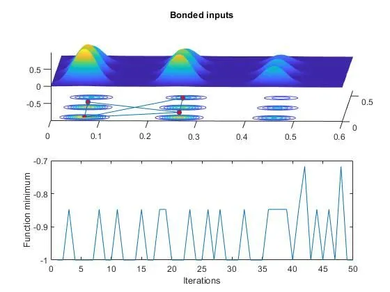
Since we are able to see the Surface graph from the first study we can assume where the Maximum will be hence so we will be directing the algorithm to search in that region.

You can see that after we applied the Lower and Upper bound the results are much better. The Algorithm has reduced down the Global maxima between 4 points. This is because we have reduced the search space. This result is okay considered to the previous result but we need to find only the single global maxima.

Study 3:

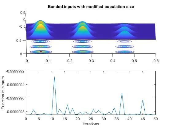
In this case study, we will be increasing the population number from 50 which is the default value to 170. The higher the number of the population it increases the probability of us finding the optimum function.

There are several things to be kept in mind when dealing with GA population :

The diversity of the population should be maintained otherwise it might lead to premature convergence.

The population size should not be kept very large as it can cause a GA to slow down, while a smaller population might not be enough for a good mating pool. Therefore, an optimal population size needs to be decided by trial and error.

So in this case the Population is 170 and the other values are the same as of the second case study. So the time taken to run the program will be more for this case.

Code:

clear all
close all
clc

x = linspace(0,0.6,150);
y = linspace(0,0.6,150);

num_cases = 50


% Creating a 2Dimensional mesh
[xx,yy] = meshgrid(x,y)


% Logic
for i = 1:length(xx)
for j = 1:length(yy)
input_vector(1) = xx(i,j)
input_vector(2) = yy(i,j)
f(i,j) = stalagmite_1(input_vector)
end
end
 tic
% Study 1 - Satistical behaviour
for i = 1:num_cases
    [inputs, fopt(i)] = ga(@stalagmite_1, 2);
    xopt(i) = inputs(1);
    yopt(i) = inputs(2);
end

study_time = toc

figure(1)
subplot(2,1,1)
hold on
surfc(x, y, -f)
shading interp
plot3(xopt,yopt,fopt,'marker','o','markersize',5,'markerfacecolor','r')
title('Unbonded inputs')
subplot(2,1,2)
plot(fopt)
xlabel('Iterations')
ylabel('Function minimum')

tic
% Study 2 - Stastical behaviour - with upper & lower bounds
for i = 1:num_cases
    [inputs, fopt(i)] = ga(@stalagmite_1,2,[],[],[],[],[0;0],[0.6;0.6]);
    xopt(i) = inputs(1);
    yopt(i) = inputs(2);
end
study2_time = toc

figure(2)
subplot(2,1,1)
hold on
surfc(x, y, -f)
shading interp
plot3(xopt,yopt,fopt,'marker','o','markersize',5,'markerfacecolor','r')
title('Bonded inputs')
subplot(2,1,2)
plot(fopt)
xlabel('Iterations')
ylabel('Function minimum')

% Study 3 increaing GA iterations
options = optimoptions('ga');
options = optimoptions(options,'PopulationSize', 170);


tic
for i = 1:num_cases
    [inputs, fopt(i)] = ga(@stalagmite_1,2,[],[],[],[],[0;0],[0.6;0.6],[],[],options);
    xopt(i) = inputs(1);
    yopt(i) = inputs(2);
end

study3_time = toc
figure(3)
subplot(2,1,1)
hold on
surfc(x, y, -f)
shading interp
plot3(xopt,yopt,fopt,'marker','o','markersize',5,'markerfacecolor','r')
title('Bonded inputs with modified population size')
subplot(2,1,2)
plot(fopt)
xlabel('Iterations')
ylabel('Function minimum')





function f = stalagmite_1(input_vector)
x1 = input_vector(1);
y1 = input_vector(2);
f1 = (sin((5.1*pi*x1)+0.5)).^6;
f2 = (sin((5.1*pi*y1)+0.5)).^6;
f3 = exp((-4*(log(2))*(x1-0.0667).^2)/0.64);
f4 = exp((-4*(log(2))*(y1-0.0667).^2)/0.64);
f = -(f1.*f2.*f3.*f4)
end

Output:

Errors faced:

No errors occured

References:

https://in.mathworks.com/help/gads/ga.html

https://en.wikipedia.org/wiki/Genetic_algorithm

Week 4.1 - Genetic Algorithm

Stopping Criteria:

Ship work like this
in your own course.

Talk to a career counsellor

Stopping Criteria:

Ship work like thisin your own course.

Talk to a career counsellor

Ship work like this
in your own course.