Week 7 State of charge estimation

AIM:

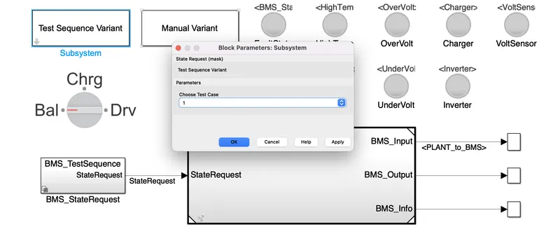
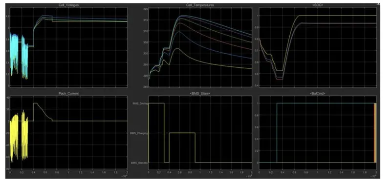
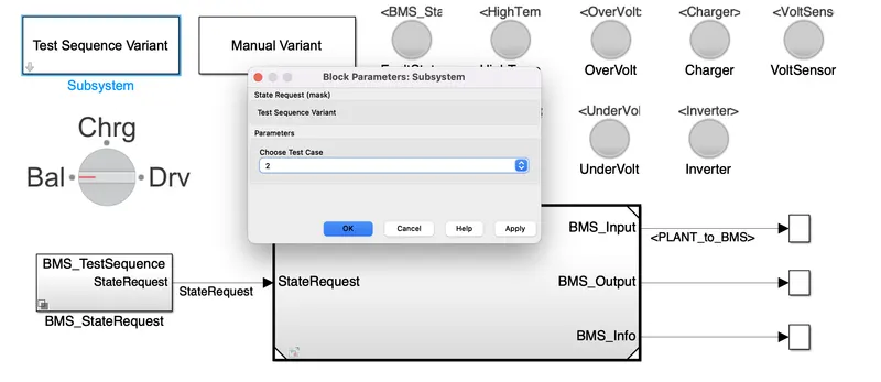
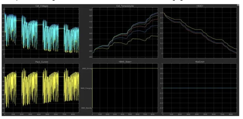
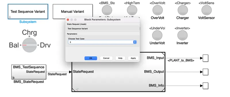
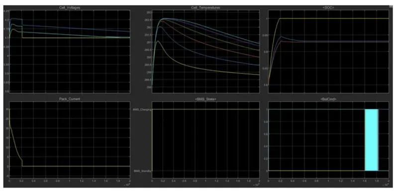
Simulate the 3 test cases from harness dashboard and write a detailed report on the results

A comparative study of LSA, BSA, G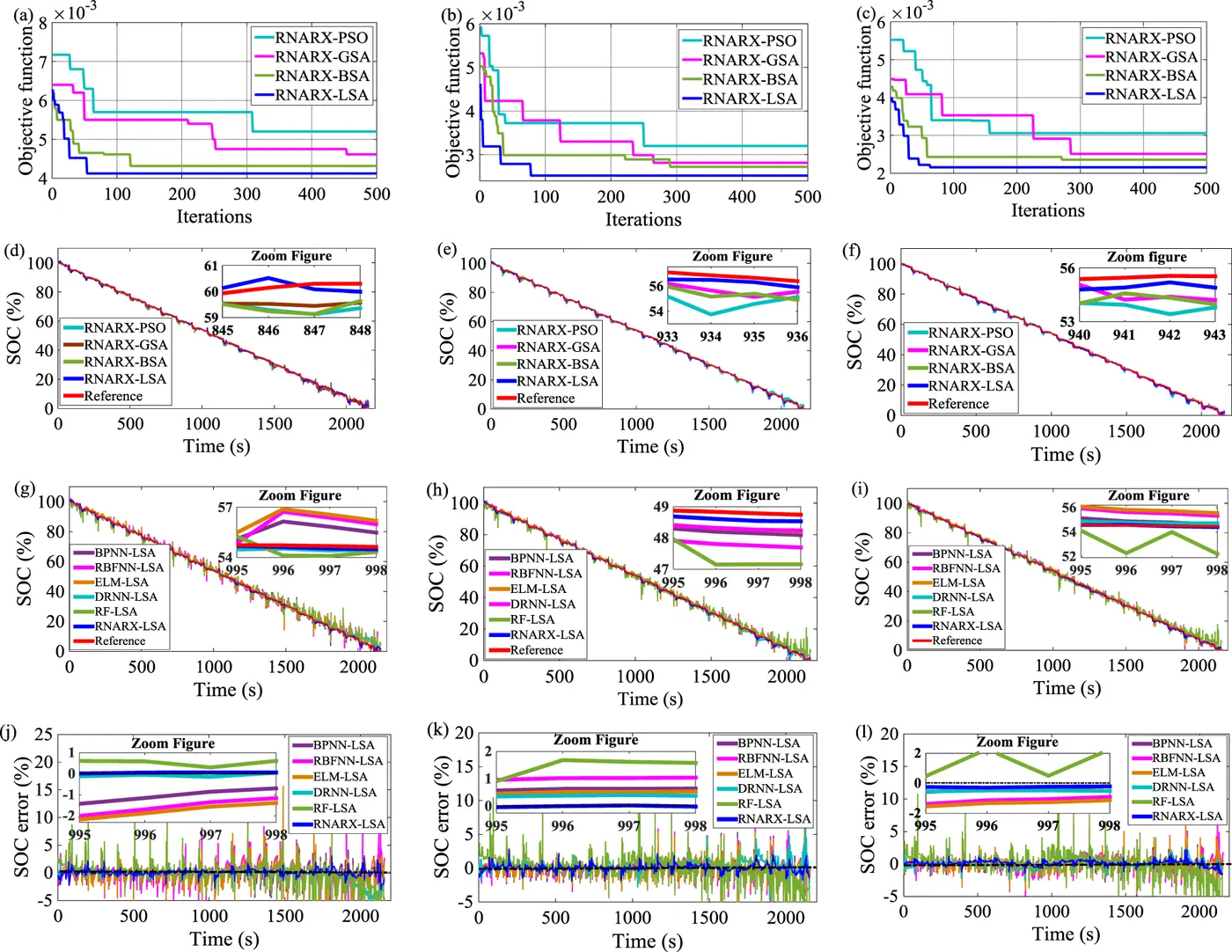SA, and PSO is conducted by developing the optimization response curve and associated objective function values, as shown in Fig. 2. The performance of LSA is superior in the HPPC load profile, where LSA achieves the lowest value of the objective function compared with BSA, GSA, and PSO. The lowest value of the objective function is estimated to be 3 × 10⁻³ after 67 iterations in HPPC 0.25 C load profile. Accordingly, IDs, FDs, and HNs related to the said iteration are computed to be 7, 2, and 10, respectively. Similar processes are used in other HPPC load profiles. The LSA results achieved from optimization response curves support the SOC estimation results. The RNARX-LSA-based SOC estimation results are found to be located near to the actual SOC values, whereas the SOC estimation results examined by RNARX-BSA, RNARX-GSA, and RNARX-PSO deviate from the reference SOC values. In HPPC 0.25 C load profile, the RMSE in RNARX-LSA is low and estimated to be 0.4302%, indicating 39.1%, 29.8%, and 19.7% reductions compared with RNARX-BSA, RNARX-GSA, and RNARX-PSO, respectively. Besides, the MAE declines by 57.4%, 50.4% and 43% in comparison with RNARX-BSA, RNARX-GSA, and RNARX-PSO methods, respectively. Similar results are also obtained in HPPC 0.1 C and HPPC 0.07 C load profiles. RNARX-LSA is dominant in other LSA-optimized ML methods. In HPPC 0.25 C load profile, the mean absolute error (MAE) of RNARX-LSA is 0.2287%, indicating 43.5%, 79.8%, 86.9%, 52%, and 83.3% reductions compared with BPNN-LSA, RBFNN-LSA, ELM-LSA, DRNN-LSA, and RF-LSA, respectively. The performance of SOC is also enhanced in obtaining small RMSE, MSE, MAE, mean absolute percentage error (MAPE) and standard deviation (SD) values. In HPPC 0.1 C load profile, the RNARX-LSA has MAPE of 5.8573% which is a reduction of 10.8%, 35.2%, 36.8%, 6.5% and 36.7% in comparison with the BPNN-LSA, RBFNN-LSA, ELM-LSA, DRNN-LSA and RF-LSA methods, respectively. In HPPC 0.07 C load profile, MSE decreases by 84.8%, 95.8%, 97.6%, 56.3% and 97.4% in RNARX-LSA compared with BPNN-LSA, RBFNN-LSA, ELM-LSA, DRNN-LSA, and RF-LSA methods, respectively

CASE:1

SOC estimation of lithium-ion batteries is commonly estimated using three methods, namely, conventional, model-based, and machine learning (ML) approaches. Conventional approaches are simple but are unsuitable for online operations. The model-based methods are known as the traditional approaches which can be extremely powerful to model the behavior of lithium-ion batteries accurately. Nevertheless, both practical and theoretical concerns cause difficulty in designing a perfect model for lithium-ion battery SOC estimation. From a practical point of view, the model-based SOC estimation model needs in-depth research, laborious experiments and extended timeframe. On the theoretical side, the model-based SOC estimation methods depend on comprehensive knowledge on battery chemistry, physics and chemical reactions which is composed of many complex mathematical equations, thus leading to complications for battery model development and parameter estimation. On the contrary, the ML-based SOC estimation approaches utilize influx of data and powerful processers to estimate SOC with limited prior knowledge about battery internal characteristics and chemical reactions. However, accuracy and performance of the ML methods depend heavily on the quality and amount of the data since unbalanced data would lead to overfitting and underfitting problems.

an added filter in the data pre-processing steps rather only needs sensors to monitor the battery signals such as voltage, current, and temperature.

CASE:2

The scientific innovation of this paper is to introduce an optimized ML technique for SOC evaluation towards the advancement of sustainable EV technologies. ML techniques have received huge attention for their enhanced learning capability, generalization performance, convergence speed, and high accuracy, hence it can be ideal to address the complex and nonlinear characteristics of lithium-ion batteries. However, the hyperparameters selection of ML algorithms by inefficient trial and error leads to computation complexity, such as slow training speed and data fitting problem, thereby delivering unsatisfactory SOC results. Currently, the optimization techniques have been increasingly popular to achieve high adaptability, improved efficiency, and high-quality results thus can be employed to determine the optimal hyperparameters as well as appropriate training algorithm, and activation function of ML algorithms. Therefore, a proper combination of ML algorithm and optimization technique not only resolves the computational complexity of ML algorithms but also achieves excellent solutions in lithium-ion battery SOC estimation.

updates the learning parameters including weights and bias by self-learning algorithm while using the past and present information of the input layer along with past information of the output layer to examine SOC. In contrast, the model-based SOC estimation is designed based on the deep understanding and knowledge of the lithium-ion battery background processes.

CASE-3

RESULT:

he optimization response curves are generated for the FUDS drive cycle, and the minimum value of objective functions is noted to obtain the best value of hyperparameters of the RNARX algorithm. The optimization performance comparison of LSA, BSA, GSA, and PSO under three different temperatures is displayed in Fig. 4. LSA achieves the lowest value of objective function among all optimization techniques, achieving 5.89 × 10⁻³, 4.17 × 10⁻³, and 3.49 × 10⁻³ after 29, 34, and 67 iterations, respectively. The corresponding iterations deliver the appropriate value of IDs, FDs, and HNs of 4, 1, 15; 2, 2, 18, and 3, 2, 17 at 0 °C, 25 °C, and 45 °C, respectively. The RMSE, and MAE, values ensure the superiority of RNARX-LSA performance compared with RNARX-BSA, RNARX-GSA, and RNARX-LSA. The MAE of RNARX-LSA at 0 °C decreases by 42.9%, 35%, and 13.8% compared with RNARX-BSA, RNARX-GSA, and RNARX-PSO, respectively. RNARX-LSA has lower RMSE, MSE, MAE, MAPE, SD values than that of BPNN-LSA, RBFNN-LSA, ELM-LSA, DRNN-LSA, and RF-LSA. At 25 °C, the RMSE of the proposed method decreases by 89.4%, 92%, 91.7%, 62.6%, and 91.7% compared with BPNN-LSA, RBFNN-LSA, ELM-LSA, DRNN-LSA, and RF-LSA, respectively. Similarly, at 25 °C, MAPE declines by 58.5%, 62%, 53.2%, 41.7% and 51.8% in comparison with BPNN-LSA, RBFNN-LSA, ELM-LSA, DRNN-LSA, and RF-LSA, approaches respectively. It is also reported that the change in temperature affects the SOC estimation results. For example, at 0 °C, MAE is achieved to be 0.58% in the proposed method which is a rise of 15.4% and 54.8% form the value obtained at 25 °C and 45 °C, respectively. Likewise, at 25 °C, RMSE, MSE, MAPE, and SD values increase by 38.9%, 50.2%, 72.1%, and 39.6%, compared with the values derived at 45 °C, respectively. The SOC error is also found narrow and remained under ±5%, ±4%, and ±2% at 0 °C, 25 °C, and 45 °C, respectively

AIM: coulomb counting BMS implements coulomb counting for SOC estimation

⇨ coulomb counting

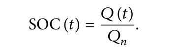
Consider the speedometer and odometer in a car. The speedometer is like an ammeter - it shows you your instantaneous speed, which is good to know, but it can't tell you how far you've gone unless you're constantly keeping track of it. This is the odometer's job; it constantly monitors your speed, accumulates it over time, and tells you how far you've traveled.

A coulomb counter is like an odometer for current. It constantly monitors the current your circuit is using, adds it up, and gives you a pulse each time a given amount of amp-hours have been used. With each pulse, you'll also get a "polarity" signal, which tells you which direction the current is flowing (great for rechargeable batteries!). By counting the pulses and direction, you can maintain an accurate count of how much power your circuit is removing from (or putting back into) your battery. If you start with a full battery, you'll always know exactly how much of it is left! Neat

he state transition equations for the battery model are given by:

where and are the thermal and SOC-dependent resistor and capacitor in the RC block, is the voltage across capacitor , is the input current, is the battery temperature, is the battery capacity (unit: Ah), and is the process noise.

The input currents are randomly generated pulses when the battery is discharging and constant when the battery is charging.

To use the Unscented Kalman Filter block, you specify the measurement and state transition functions using either Matlab or Simulink functions. This example demonstrates the use of Simulink functions. Since Unscented Kalman Filters are discrete-time filters, first discretize the state equations. In this example, Euler discretization is employed. Let the sampling time be . For a general nonlinear system , the system can be discretized as:

The state vectors of the nonlinear battery system are:

.

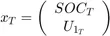Applying Euler discretization gives the following equations:

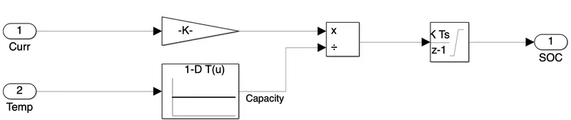
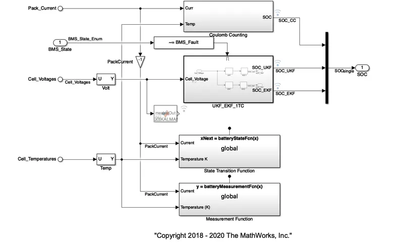
The discretized state transition equation is implemented in the Simulink function named batteryStateFcn. The function input x is the state vector, and the function output xNext is the state vector at the next step, calculated using the discretized state transition equations. In the function, you need to specify the signal dimensions and data type of x and xNext. In this example, the signal dimension for x and xNext is 2, and the data type is double. Additional inputs to batteryStateFcnare the temperature, estimated capacity, and current. Note that the additional inputs are inputs to the state transition equations and are not required by the Unscented Kalman Filter block.

The nth-order Thevenin model is widely used for SOC estimation because of its relatively high accuracy and computation efficiency compared with other models [1]. Increasing the order of the Thevenin model will improve the model accuracy further. However, higher order result in additional calculation cost [17]. In the paper, a 2nd-order RC model as shown in Fig. 1 is employed to estimate the dynamic characteristics of the battery. The voltage source UOCV represents the battery OCV. ro is the internal ohmic resistance. The parallel RC network consists of rp1 and cp1 is aimed to model the fast dynamic voltage of the battery. Similarly, the parallel RC network consists of rp2 and cp2 is aimed to model the slow dynamic performance. Up1 and Up2 represent the polarization voltages across the two RC networks, respectively. Uo and I are the terminal voltage and load current, respectively. The electrical behavior of the battery can be expressed as follows.

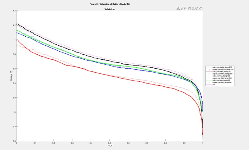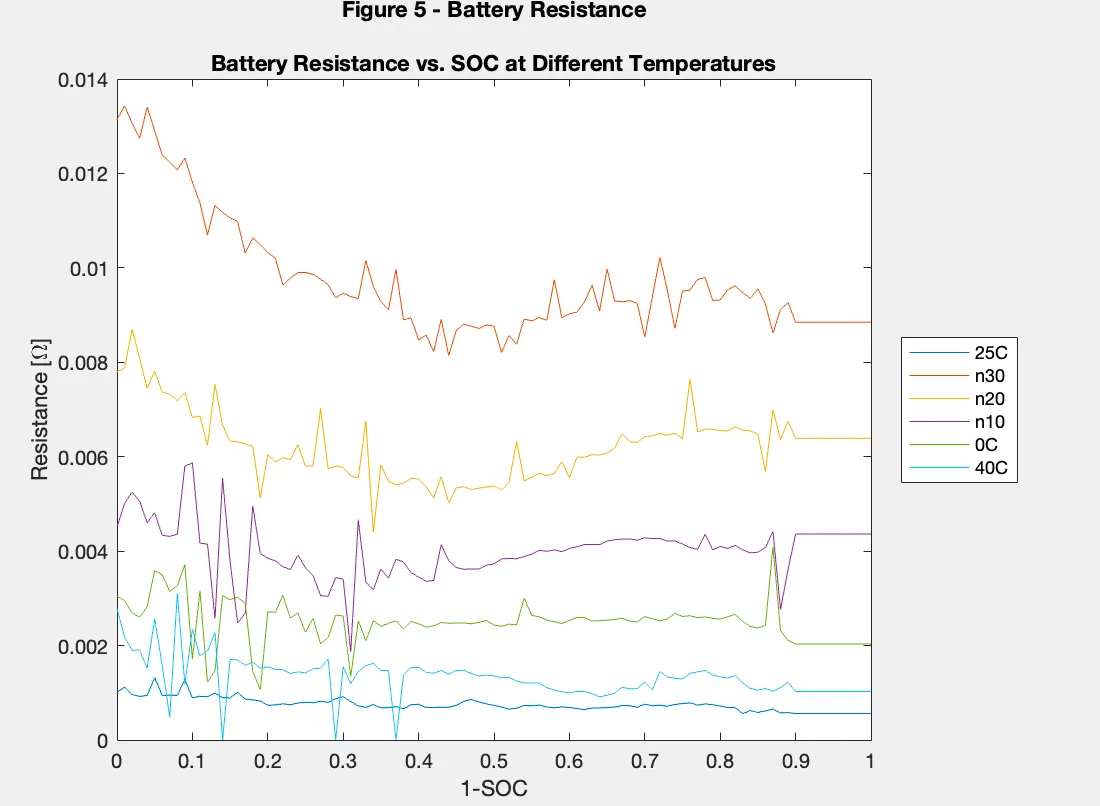
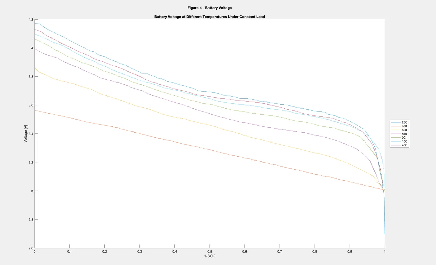
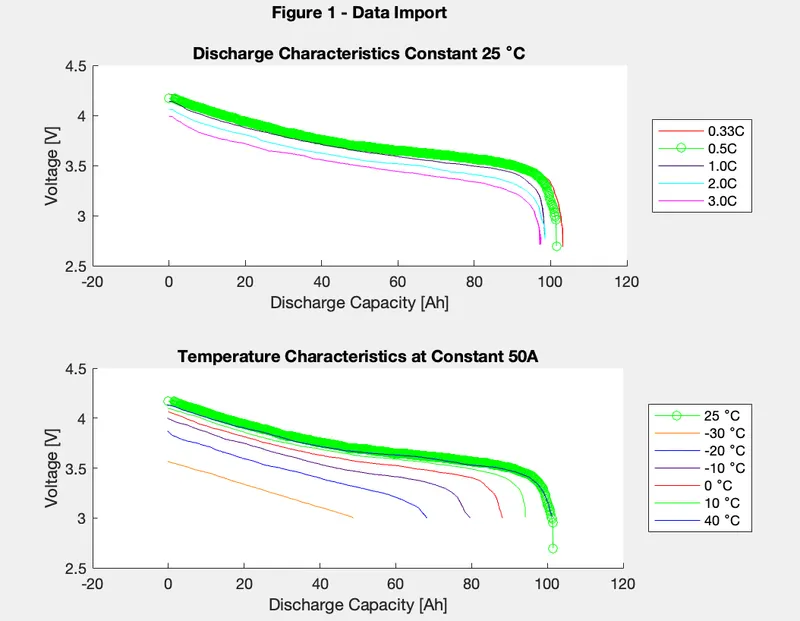
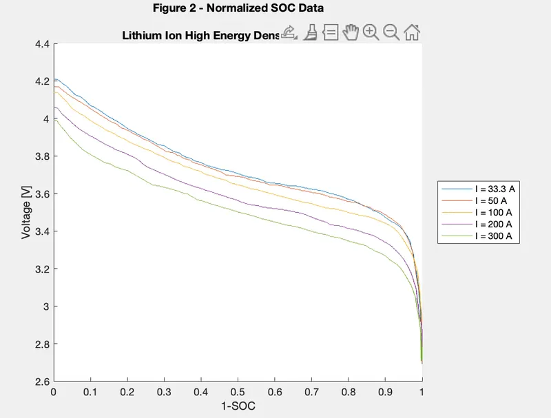
RESULT: SOC under different discharging conditions. Four categories of estimating mathematical methods, which have their own characteristics, were discussed. Papers were selected to emphasize the diversity of estimating mathematical methods. Some of these methods have good performances at fixed discharging current condition, while others perform better in varied discharging current condition. It is difficult to evaluate the performance of various methods, as the existing applications were in different discharging condition and different size of battery. The developments of various SOC estimate methods are expected to be valuable in battery applications such as BMS in hybrid electric vehicles. Based on the development history of SOC estimation, the future development directions of SOC estimating are proposed in the end.