Week 7 State of charge estimation
Aim:
- To simulate the 3 test cases from the harness dashboard and write a detailed report on the results
- What is coulomb counting? Refer to the above model and explain how BMS implements coulomb counting for SOC estimation?
- Simulating the 3 test cases from the harness dashboard and writing a detailed report on the results
1. To simulate the 3 test cases from the harness dashboard and write a detailed report on the results.
Answer:
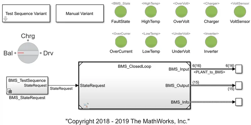
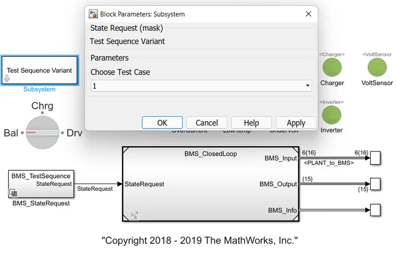
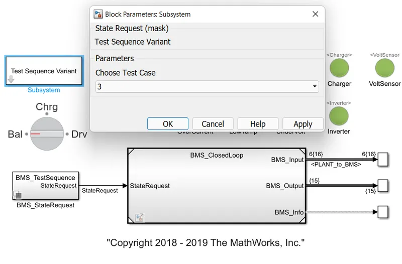
The above figure is obtained by the link provided with the problem system itself and given in reference no.1. With the help of the Test Sequence Variant, the Test case sequence are changed to 1, 2 and 3 simulated each one at a time.
Test Sequence 1:
Test Sequence 1 Report:
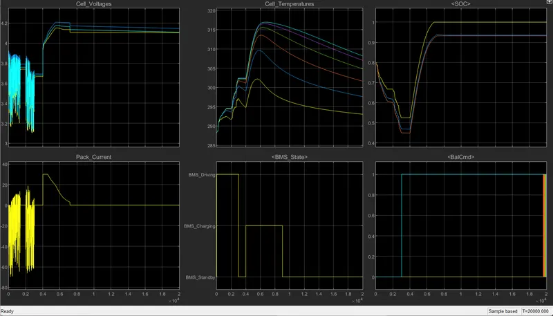
The above graph indicates 6 different grasp that are Cell Voltages, Pack Current, Cell Temperature, BMS Status, SOC using 3 different methodologies and Cell Balance Command Signals.
In the first graph, Cell voltages changes in values as the current is going in and out of the cell by charging and discharging it respectively. At first, we can observe that the voltage values of the cells differ in values slightly, it is because we initialized the model with a slight imbalance between the given cells. For 0 to 3000 seconds the cell voltages range between 3.1 to 3.9V (Driving part) approximately and then balances for a very short amount of time to the nominal values of 3.7V. Later, cell voltage touches the 4.2V mark by sudden rise (Charging state) behaviour and ultimately settles down to a lower value, at the end of the simulation. At that time the cell voltage tries to converge to each other values with the balancing methodology and ends up between the 4 to 4.2V range.
The second graph shows the current rating of the battery pack which basically defines the current characteristics of all the cells as a whole. In driving mode, the pack current has the ranges from -70 Amps at the time of charging (the charging current is taken as positive here) and then stays zero at the time of standby balanced mode for the rest of the simulation, giving zero value due to zero power demands.
The third graph is showing us the cell temperatures for all the cell voltages. When the BMS is in driving mode, the cell temperature rises due to the different power demands of the drive cycles. The balanced mode happens for a very short duration; it tries to converge, but the window is of very little time they cannot converge. After that when the charging state comes, all the cell temperature rises and after a point (5550 seconds) it again starts to decrease due to the balancing effect but a decrease in pack current. The clear difference between the hottest cell (No.6) and the coldest cell (No.1) is because of the underperforming cell. Cell No.6 is significantly hotter the cell no.1 because it is thermally insulated on one side. The higher temperature of cell no.6 will eventually cost much faster degradation of cell 6 compared to cell 1 leading to undesirable and unevenness in cell conditions. Therefore, need an active thermal management system to keep thermal differences within a few degrees Celsius so that the performance of the battery pack is not compromised.
The fourth graph gives us an idea about the BMS state which is the vehicle undergoing that are Driving, Charging and Standby mode or Balance mode.
In the fifth graph, the SOC of three different battery cells each performing with different matter yellow corresponds to column counting, blue corresponds to UKF and orange to EKF, the initial SOC is 75%, however, the simulation so estimates need to initialize 80% to set their capability to recover. It is apparent that coulomb counting never does because it has no way to realize it due to the absence of voltage information. Both common filter algorithms on the other hand recover from the initial error within the first hour of simulated time. Here, EKF slightly outperformance UKF.
The sixth graph gives us the balance commands of the cells. We can see here that from the falling edge of the BMS driving mode, the balance command is initiated for all the batteries except cell no.1 which is the closest. It is because, from this point in time, all the cell's temperature significantly increases and crosses a certain difference with the temperature of cell no.1.
Test Sequence 2:
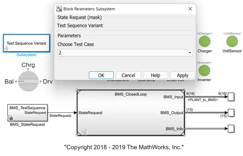
Test Sequence 2 Report:
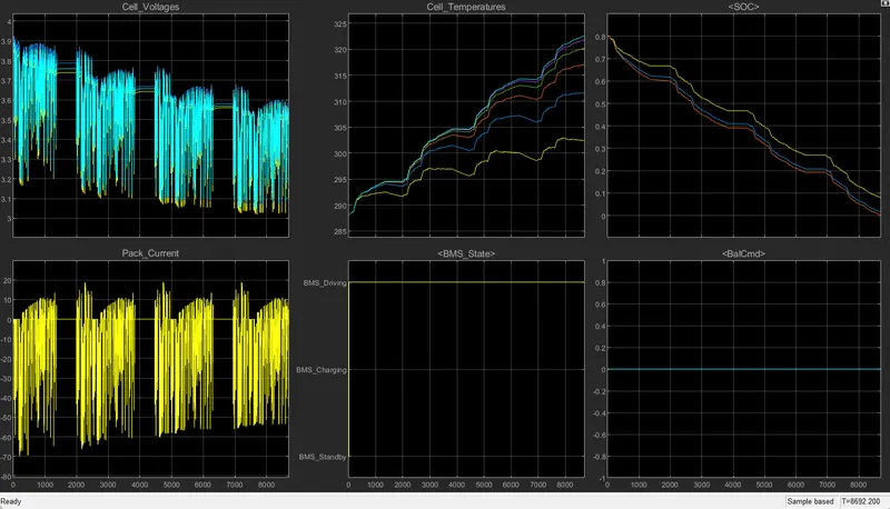
The fourth graph shows us that the simulation is run throughout the BMS driving mode.
In graph 1, the initial state the voltage of all the cells is deflecting in the same manner and dropping slightly in the range of 3 to 3.9V. It has 4 fluctuation zones and in between each of these fluctuating zones, they are stable for a while and this phase lasts for 8500 sec.
Graph 2 also shows us the same behaviour as the voltages, but it has negative values most of the time whenever the higher voltage drop is required and a -70A to 20A value like before.
The temperature graph here is showing us all the cells’ temperatures were the same at the start of the simulation which is 288 degree-kelvin. Here, temperature discrepancies are also observed between each cell. Cell no.6 is the hottest and cell no.1 is the coldest like before and the temperature difference here is 20 degrees approx. This can easily degrade the overall performance of the battery pack.
The SOC of three different battery cells each performed with different matter yellow corresponds to coulomb counting, blue corresponds to UKF and orange to EKF, the initial SOC is 75%, however, the simulation so estimates need to initialize it to 80% to set their capability to recover. It is apparent that coulomb counting never does because it has no way to realize it due to the absence of voltage information. Both common filter algorithms on the other hand recover from the initial error within the first hour of simulated time.
The SOC for all three values is decreasing from 80% of the value and continuously decreases because the entire simulation is in driving mode. Coulomb counting soc value decreases at a lesser rate than the other two, where UKF shows even lesser than EKF.
The balance command is not initiated for any of the cells for this specific simulation. That may be since for continuous driving mode this much difference or disbalance can be allowed because no overcharging will be taking place.
Test Sequence 3:
Test Sequence 3 Report:
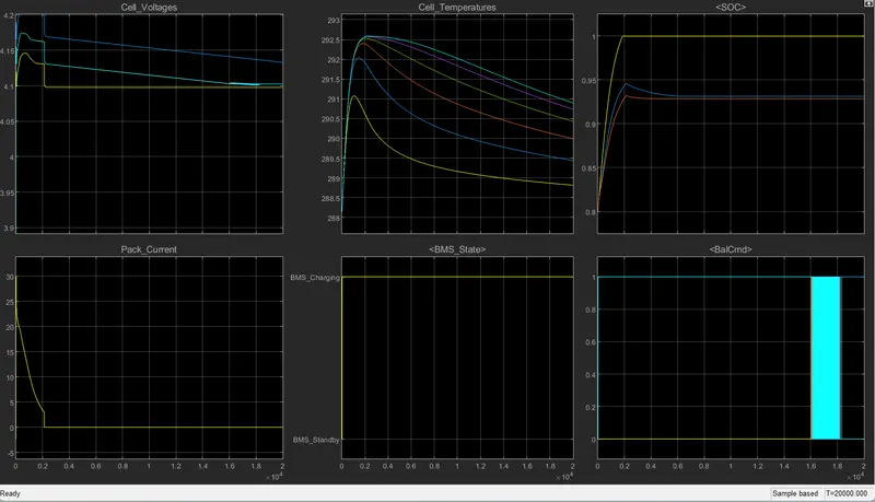
The fourth graph clearly shows that the entire simulation is based on the charging mode.
From the first graph, all the cells are initiated at different voltages where cell no. 2 has the lowest voltage. After some time, cell number 8 quickly comes near the cell number 1 voltage value whereas there is a significant difference in the cell number 2 voltage.
The pack current shows a higher charging current at the initiation of the simulation but as time goes the pack current decreases and becomes zero at the end. The battery pack current is initiated with 20 A and then it falls to zero current till its complete simulation time of 2000 sec then it maintains the constant current because it is put in a charging state and it remains constant throughout the simulation.
The cells initiate with 287 degree-kelvin and then all the cells maintain the straight line but with different temperatures range. In the end, all the cells have a different temperature) traces show the significant discrepancy between the hottest and coldest cells the reason is mainly because of symmetry in the merger layer in terms of thermal behaviour it is thermally insulated on one side.
The SOC is the initial SOC of three different cells is at 80%. As the system is put in a charging state, the SOC rises to 100% for the yellow cell, UKF and EKF initially have different charging rates but after 4000 sec they have an equal state of charge of 91% and it maintains throughout the simulation. It is apparent that coulomb counting never does because it has no way to realize it, making it erroneous due to the absence of voltage information. Both common filter algorithms on the other hand recover from the initial error. EKF and UKF slightly outperform the coulomb counting.
The balance commands of the cells, we can see from the sixth graph. The command for cell no.1 is never initiated because it is the coldest but for the other cells, it is initiated from the beginning. When after 16000 seconds the voltage temperature comes close enough to each other the balance command for all the other cells is reset to the 0 value at 18000 seconds. Between this time, the command status changes rapidly from 1 to 0 by constantly monitoring the temperatures and ultimately falls to zero when the temperature difference becomes very less.
2. What is coulomb counting? Refer to the above model and explain how BMS implements coulomb counting for SOC estimation?
Answer:
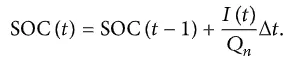
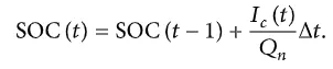
By the coulomb counting method, the discharging current of a battery is measured and integrates the discharging current over time to estimate SOC. Coulomb counting method is done to estimate the SOC(t), which is estimated from the discharging current, I(t), and previously estimated SOC values, SOC(t-1). SOC is calculated by the following equation:
But several factors affect the accuracy of the coulomb counting method including temperature, battery history, discharge current, and cycle life. To improve this, Modified Coulomb Counting is used.
To improve the coulomb counting method, a new technique called the Modified Coulomb Counting method is proposed. The modified Coulomb counting method uses the corrected current to improve the accuracy of estimation. The corrected current is the function of discharging current. There is a quadratic relationship between the corrected current and discharging current of the battery. By the practice of experimental data, the corrected current is calculated in the following form:

Where, k1, k2, and k0 are constant values obtained from the practice experimental data.
In the modified Coulomb counting method, SOC is calculated by the following equation:
Flowchart for Coulomb Counting Method
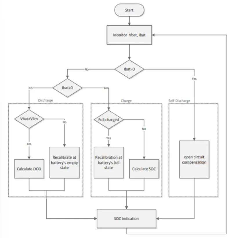
The flowchart given in Fig above explains the algorithm used to manage the battery monitoring by switching from a battery operating mode to another to the conditions of the transition. The estimation of the SOC of a Li-ion battery in this method is based on monitoring both the voltage Vbat and the current Ibat. The operation mode of the battery is recognized by the direction of current through the battery system. When the battery is in open circuit mode, Ibat = 0 and compensation of self-discharge losses will be taken into account as explained in sub-section C. The information needed to carry out monitoring is the measurement of the battery voltage, the current flowing through it, and the operating temperature. Coulomb counter ∆Q is used to track the SOC when the battery is charged or discharged.
The number of charges ∆Q in an operating period ‘T’ is obtained by temporal integration of a measured charging/discharging current Ibat like expressed in (2)

This variance ∆Q that will be used in the following equations is negative if the battery is in discharge, positive if in charge.
(I). Charge mode
In this mode, the coulomb counter is presented by Qgained as expressed in (3), which represents the number of charges accumulated during ‘T’

So, the variation of the state of charge gained in this same operating period is obtained by the relation (4)

By cumulating the previous state of charge indication and the obtained one we can have the instantaneous value of SOC.

Knowing the relationship indicated about (6) the value of depth of discharge DOD is updated in every charging operation to get it back every switching to discharging mode.

(II). Discharge Mode
In the discharge mode the coulomb counter is presented by Qlost, which represents the amount of charges losses in the operating period ‘T’ by equation (7):

The depth of discharge variation is calculated according to (8) and used in (9) to calculate the value of DOD
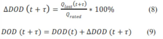
The SOC indication then is done by applying the equation (6).
(III). Self-Discharge Mode
During the battery storage periods, the percentage of monthly self-discharge is converted to the amount discharged per hour; this amount is discharged by the constant q(per/hour). Considering a 5% rate of self-discharge per month q(per/hour) is approximated to 0.0016 Ah. So, the quantity of charges dissipated in the open circuit period QOC is calculated by equation (10) representing the accumulative losses during the store hours.

h: Hour of storage
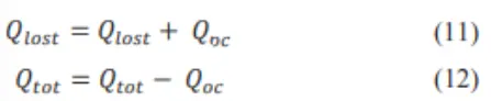
This value will be added to the amount of charge lost Qlost during discharge mode and subtracted from the amount of charge accumulated Qgained in charge mode as expressed in relations (II)and (12). This compensation of self-discharging loss is made at each open circuit period and before switching to another operating battery’s mode.
(IV). Temperature effect
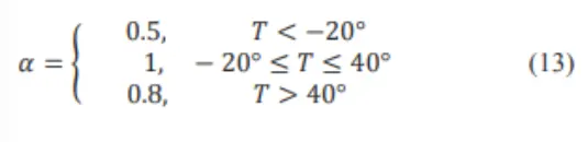
The temperature variation affects considerably the state of charge of the Li-Ion battery [16]. To improve the accuracy of the battery state of charge, a temperature coefficient 't' is introduced and multiplied by the value of the calculated SOC [17]. This coefficient varies depending on the operating temperature according to the interval’s variations (13)
(V). Recalibration
When the loaded voltage Vbat drops under a limit voltage VIim (3V), during the discharging mode the battery is considered totally charged. When it’s empty, the battery can no longer be used and should be recharged. So, after a cycle of charge/discharge, a recalibration should be made of Qmax which represents the maximum capacity that can be released by the battery. This recalibration allows rectifying the indication of SOC by replacing Qrated with Qmax in relation (4). Also, we recalibrate the state-of-Health (SOH) of the battery SOH defined is as a relation (14) as:

Moreover, the battery is fully charged. Then SOH should be updated by assigning the number of charges releasable from the battery to Qmax. The SOH indeed represents the ageing degree of the battery; in fact, it’s at 100% maximum value when the battery is new. When the battery is getting old and Qmax became more and more inferior than Qrated, the SOH value drops to indicate the health degradation of the battery.
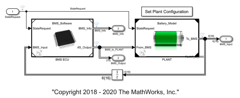
The above model is from where the SOC estimation for a Simulink model is done. The ECU does the estimation by counting what is provided and preloaded to its memory.
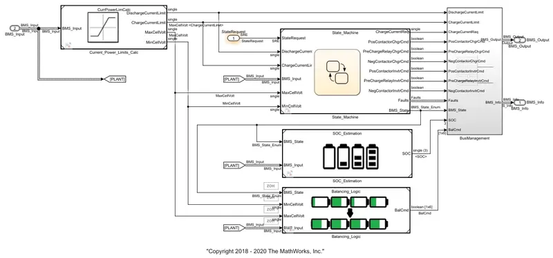
In this SOC estimation block, we can see three different techniques for the state of charge estimation. All three techniques have their own merits and limitations. The first method is coulomb counting and the other two are unscented (UKF) and extended Kalman filter (EKF). Here we are concerned with the coulomb counting method.
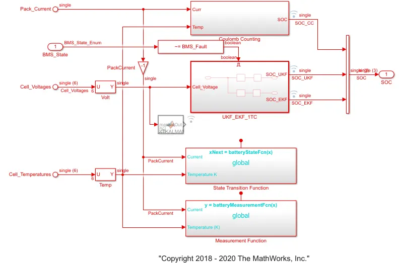
In coulomb counting method block. It takes two input signals such as current and temp and the current signal goes to gain block and the temp signal goes to lookup tables of battery time and current. And both the blocks are connected to the divided block and these signals are connected to the discrete-time integrator to track the charge and which finally helps to calculate the state of charge. This consist of integrating a current and doesn’t leave the cell for that here we use a discrete-time integrator to give the track of the cell charge time the benefit of this are its simplicity and its low capitation cost and the drawbacks are an accumulation of the current sensor error and its inability to recover from the wrong initial condition. From the lack of feedback from voltage measurements.
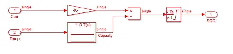
Here, the coulomb counting is done with the help of the look-up table and the discrete-time integrator block.
Conclusions:
We have simulated the 3 test cases from the harness dashboard and written a detailed report on the results.
We had knowledge of coulomb counting. Referred to the above model and explained how BMS implements coulomb counting for SOC estimation.