Week 3 - Solving second order ODEs

Aim: To write codes on MATLAB for stimulation of the Simple Pendulum.

The second-order differential equation is used to solve the simple pendulum stimulation problem.

2^nd Order Differential Equation

d²Θ/dt² + (b/m)*(dΘ/dt) + (g/L)*sinΘ = 0

Where, b = damping, m = mass, g = gravity, L = length

Let Θ = Θ₁

dΘ/dt = dΘ₁/dt

Consider, dΘ₁/dt = Θ₂ …………①

d²Θ/dt² = d²Θ₁/dt² = (d/dt)(dΘ₁/dt) = dΘ₂/dt ………….②

d²Θ/dt² + (b/m)(dΘ/dt) + (g/L)*sinΘ = 0

d²Θ₁/dt² + (b/m)(dΘ₁/dt) + (g/L)*sinΘ₁ = 0

dΘ₂/dt + (b/m)Θ₂ + (g/L)*sinΘ₁ = 0

dΘ₂/dt = -(b/m)Θ₂ - (g/L)*sinΘ₁

_{Codes for Calling a function: ode_fucn}

function[dtheta_dt] = ode_func(t, theta, b, g, l, m)
theta1 = theta(1);
theta2 = theta(2);
dtheta1_dt = theta2;
dtheta2_dt = -(b/m)*theta2 -(g/l)*sin(theta1);
dtheta_dt = [dtheta1_dt; dtheta2_dt];
end

Codes for Stimulation of Simple pendulum:

Functions ode45 and ode_func are used for solving the problem

Parameters used are the time, theta, damping coefficient(b), acceleration due to gravity(g), length(l) and mass of the bob(m).

b = 0.5

g = 9.81 m/s

l = 0.9 m

m = 2 kg

Program to show damping effect

clear all
close all 
clc
% Inputs
b = 0.5;
g = 9.81;
l = 0.5;
m = 2;

% Initial Condition
theta_0 = [0;5];

% Time Point
% For 0 to 10 seconds time has been taken with intervals od 100
time = linspace (0,10,100);

% ODE Solver

[t,results] = ode45(@(t,theta) ode_func(t,theta,b,g,l,m),time,theta_0);

% plotting
plot(t,results(:,1))
hold on
plot(t,results(:,2))
xlabel('Position Radians')
ylabel('Angular velocity')
grid on;

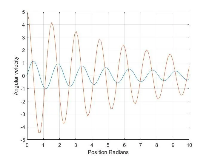
Plot of the damping effect

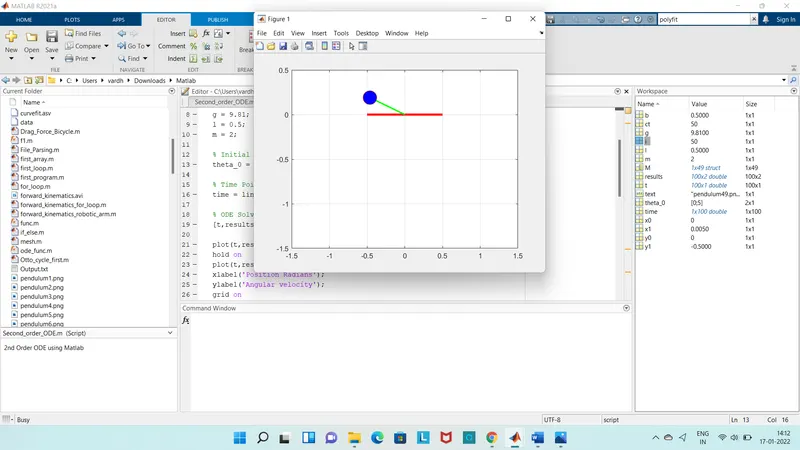
Stimulation of Simple Pendulum

clear all
close all 
clc
% Inputs
b = 0.5;
g = 9.81;
l = 0.5;
m = 2;

% Initial Condition
theta_0 = [0;5];

% Time Point
% For 0 to 10 seconds time has been taken with intervals od 100
time = linspace (0,10,100);

% ODE Solver

[t,results] = ode45(@(t,theta) ode_func(t,theta,b,g,l,m),time,theta_0);

plot(t,results(:,1))
hold on
plot(t,results(:,2))
xlabel('Position Radians')
ylabel('Angular velocity')
grid on;


% Simulation of Pendulum

ct = 1; % The simulation time is obtained by calling getCurrentTime.
for i = 1:length(results(:,1))
    x0 = 0;
    y0 = 0;
    x1 = l*sin(results(i,1));
    y1 = -l*cos(results(i,1));
    
    plot([-0.5,0.5],[0,0],'linewidth',3,'color','r');
    line([x0 x1],[y0 y1],'linewidth',2,'color','g');
    hold on;
    
    plot(x1,y1,'o','markers',20,'markerfacecolor','b');
    grid on;
    axis([-1.5 1.5 -1.5 0.5]);
    pause(0.01);
    hold off;
    M(ct) = getframe(gcf);
    text = sprintf("pendulum%d.png",ct);
    saveas(1,text);
    ct = ct +1;
end

% making video of robotic arm
movie(M)
% VideoWriter(filename,profile) additionally applies a set of properties tailored to a specific file format.
videofile = VideoWriter('pendulum_animation.avi','Uncompressed AVI')
open(videofile)
writeVideo(videofile, M)
close(videofile)

% End of the program

https://youtu.be/7oh2olMtL9o

Errors I got while doing program