Project 2 - Rankine cycle Simulator
Aim: To stimulate the Rankine Cycle and plot the corresponding T-S and H-S plots using MATLAB.
Objective:
- Calculate the state points of the Rankine Cycle based on given inputs.
- Plot the corresponding T-S and H-S plots for the given set of inputs.
Given:
Input Values:
- Turbine Inlet temperature = 400° C
- Turbine Inlet Pressure = 30 bars
- Turbine Outlet Pressure = 0.05 bars = Condenser Inlet Pressure
Required Output Values:
- NetWork Output
- Back Work Ratio
Note: The standard Xsteam library to get the steam table data for water, is given, which must be used to calculate the points in between the state variables.
What is a Rankine Cycle?
A Rankine Cycle is the most widely used thermodynamic cycle in various power plants such as nuclear power plants or coal-fired power plants. The Rankine cycle describes the procedure through that a reciprocating steam engine or a steam turbine extracts mechanical energy from the working medium when it flows between a heat reservoir and heat source.
In simple words, a Rankine cycle describes how a heat engine such as a steam engine extracts thermal energy from a heat source and uses this energy to produce electricity. These heat sources may have combustion of ethanol, biomass, oil, natural gas, coal or nuclear fission process etc.
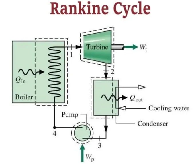
The thermal energy extraction capacity of the Rankin engine varies according to the heat sink temperature and heat source temperature.
The Ideal Rankine Cycle:
In the case of the vapour cycle, if the working medium moves over the different parts of a powerplant without any friction pressure and irreversibility loss, the cycle is referred to as the ideal Rankine cycle.
The Rankine cycle is a major working cycle of all power plants in which operating liquid changes continuously from liquid to vapour and vapour to liquid. It is a theoretical cycle in which thermal energy transforms into useful work.
A T-s diagram of the Rankine cycle is given below, which will be helpful to understand the Rankine cycle works
.
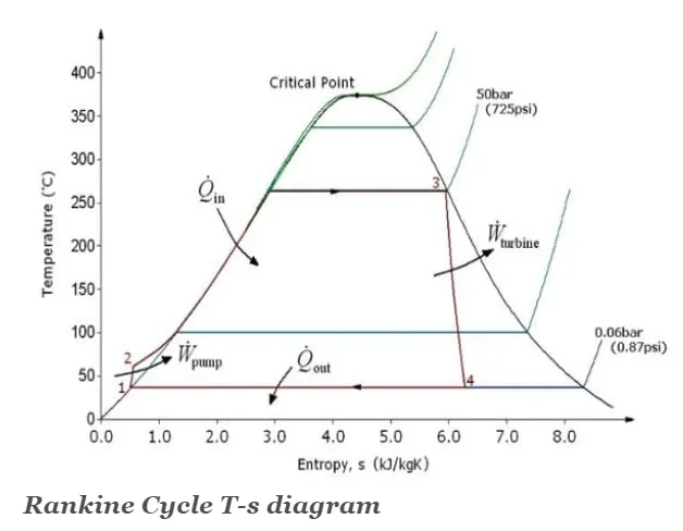
The stages of completing a Rankine cycle are given below:
- Isentropic Compression (1 to 2): In this stage, a pump uses to transfer the water or other working medium from the water body (canal or tank etc.) into the boiler. The pump requires a small amount of energy for initial pumping. It pumps the fluid by increasing the pressure of the fluid, but fluid entropy remains the same.
- Constant Pressure Heat Addition Process (2 to 3): As the water is delivered into the boiler, an external heat source provides heat to the boiler. The boiler heated the water at constant pressure and converts it into dry saturated vapour (steam). During this process, the enthalpy of the liquid changes, and pressure remains constant.
- Isentropic Expansion (3 to 4): After the constant pressure heat addition process, the steam enters into the turbine area, where it expands. As the steam expands, it strikes with the turbine blades, which convert the thermal energy of the steam into rotational energy (mechanical work). As the turbine blades are rotated, they also rotate a crankshaft that further rotates the coil of the generator. As the coil rotates in a magnetic field, it produces electricity. During this whole process, the pressure and temperature of the steam decrease; due to that, some condensation can happen.
- Constant Pressure Heat Rejection Process (4 to 1): The vapour or steam enters the condensate tank after the expansion process. In this condensation process, the vapour is condensed to convert into saturated liquid. During this process, the vapour rejects heat, but its liquid pressure remains the same.
In an ideal Rankine cycle, the turbine and pump work under isentropic conditions. It means the turbine and pump don’t generate entropy; they just increase the performance of the cycle.
The Rankine cycle (shown in the above diagram) avoids the working medium ending up in the superheated vapour area after expanding in the turbine, which decreases the energy dissipated by the condenser.
Procedure:
All required variables and parameters have to be calculated.
Using the 'XSteam' library function, all the parameters have to be sorted out.
The usual calculations and plotting of the graphs were done as per the theory of thermodynamics.
MATLAB Program:
% Rankine Cycle Stimulator
clear all
close all
clc

% Printing Introduction
fprintf(        'RANKINE CYCLE SIMULATOR        \n') % Title for results
fprintf('\n1-2 is Isentropic Expansion in the Turbine \n')
fprintf('2-3 is Constant Pressure Heat Rejection by the Condenser \n')
fprintf('3-4 is Isentropic Compression in Pump \n')
fprintf('4-1 is Constant Pressure Heat Addition by the Boiler \n')

% User Inputs
P1 = input('\nEnter the Pressure at the Turbine Inlet (in bar): \n');
T1 = input('Enter the Temperature at the Turbine Inlet(in °C): \n');
P2 = input('Enter the Pressure at the Turbine Inlet (in bar): \n');

% State Point 1
% XSteam() is the MatLab program in which values are taken
H1 = XSteam('h_pT',P1,T1); % Enthalpy
S1 = XSteam('s_pT',P1,T1); % Entopy
Hf1 = XSteam('hL_p',P1); % Enthalpy of Saturated Liquid
Hg1 = XSteam('hV_p',P1); % Enthalpy of Saturated Vapour
Ts1 = XSteam('Tsat_p',P1); % Saturation Temperature
Sf1 = XSteam('sL_p', P1); % Entropy of Staurated Liquid
Sg1 = XSteam('sV_p', P1); % Entropy of Staurated Vapour

% Sate Point 2
S2 = S1;
Sf2 = XSteam('sL_p', P2);
Sg2 = XSteam('sV_p', P2);
x = (S2-Sf2)/(Sg2-Sf2); % Deyness Fraction
Hf2 = XSteam('hL_p',P2);
Hg2 = XSteam('hV_p',P2);
H2 = Hf2 + x*(Hg2-Hf2);
T2 = XSteam('T_ph',P2,H2);
Ts2 = XSteam('Tsat_p',P2);

% State Point 3
H3 = Hf2;
S3 = Sf2;
T3 = T2;
P3 = P2;

% State Pont 4
P4 = P1;
S4 = S3;
H4 = XSteam('h_ps',P4,S4);
T4 = XSteam('T_ps',P4,S4);

t = linspace(0,374,500); % Temp Space fpr Plotting Saturation Curves

% Plot T-S Diagram
figure(1)
hold on
% plot Saturation Curve
for i = 1:length(t)
    plot(XSteam('sL_T',t(i)),t(i),'.','color','b')
    plot(XSteam('sV_T',t(i)),t(i),'.','color','b')
end
% Plot Cycle
plot([S1 S2],[T1 T2],'linewidth',2,'color','r')
if x>1
    T3 = Ts2;
    plot([S2 Sg2 S3 S4],[T2 Ts2 T3 T4],'linewidth',2,'color','r')
    T2 = Ts2;
else
    plot([S2 S3 S4],[T2 T3 T4],'linewidth',2,'color','r')
end
l = linspace(T1,T2,1000);
for i = 1 : length(l)
    plot(XSteam('s_pT',P1,l(i)),l(i),'.','color','r')
end
plot([Sf1 Sg1],[Ts1 Ts1],'linewidth',2,'color','r')
xlabel('Entropy(kJ/kg-K)')
ylabel('Temperature(K)')
title('T-S Diagram')
text(S1,T1,'1') % text() is used for giving the location number
text(S2,T2,'2')
text(S3,T3,'3')
text(Sf1,Ts1,'4')

% Plot H-S Diagram
figure(2)
hold on
% Plot Saturation Curve
for i = 1:length(t)
    plot(XSteam('sL_T',t(i)),XSteam('hL_T',t(i)),'.','color','b')
    plot(XSteam('sV_T',t(i)),XSteam('hV_T',t(i)),'.','color','b')
end
% Plot Cycle
plot([S1 S2 S3 S4 S1],[H1 H2 H3 H4 H1],'linewidth',2,'color','r')
xlabel('Entropy(kJ/kg-K)')
ylabel('Enthalpy(kJ/kg)')
title('H-S Diagram')
text(S4,H4,'   ,4')
text(S3,H3,' 3')
text(S2,H2,'2')
text(S1,H1,'1')

% Calculation
% Turbine Work
Wt = H1-H2;

% Pump Work
Wp = H4-H3;

% Heat Addition
Qin = H1-H4;

% Heat Rejection
Qout = H2-H3;

% NetWork
Wnet = Wt-Wp;

% Efficiency
Ntherm = (Wnet/Qin)*100;

% Specific Steam Consumption
SSC = 3600/Wnet;

% Back Work Ratio
BWR = Wp/Wt;

% Print Result
% fprintf() is used to print the  line in result in command windows
fprintf('\n \n Results\n')
fprintf('At State Point 1:\n')
fprintf('P1 is : %.2f bar\n',P1)
fprintf('T1 is : %.2f °C\n',T1)
fprintf('H1 is : %.2f kJ/kg\n',H1)
fprintf('S1 is : %.2f kJ/kg-K\n',S1)


fprintf('\nAt State Point 2:\n')
fprintf('P2 is : %.2f bar\n',P2)
fprintf('T2 is : %.2f °C\n',T2)
fprintf('H2 is : %.2f kJ/kg\n',H2)
fprintf('S2 is : %.2f kJ/kg-K\n',S2)

fprintf('\nAt State Point 3:\n')
fprintf('P3 is : %.2f bar\n',P3)
fprintf('T3 is : %.2f °C\n',T3)
fprintf('H3 is : %.2f kJ/kg\n',H3)
fprintf('S3 is : %.2f kJ/kg-K\n',S3)

fprintf('\nAt State Point 4:\n')
fprintf('P4 is : %.2f bar\n',P4)
fprintf('T4 is : %.2f °C\n',T4)
fprintf('H4 is : %.2f kJ/kg\n',H4)
fprintf('S4 is : %.2f kJ/kg-K\n',S4)

fprintf('\nTurbine Work(Wt) is : %.2f kJ/kg\n',Wt)
fprintf('Pump Work(Wp) is : %.2f kJ/kg\n',Wp)
fprintf('Wnet is : %.2f kJ/kg\n',Wnet)
fprintf('Thermal Efficiency is : %.2f %\n',Ntherm)
fprintf('Specific Steam Consumption(SSC) is : %.2f kg/kWh\n',SSC)
fprintf('Back Work Ratio is : %.3f \n',BWR)
End of the program
Steps:
1. Start the program with the 'clear all', 'close all' and 'clc' commands.
2. The 'input()' command is used to take the user input. The input includes the Temperature, Pressure before entry to the turbine and Pressure after exiting from the turbine.
3. Based on input parameters at 4 State Points are calculated.
Thermodynamic parameters include Enthalpy (H), Entropy (S), Temperature (T), Pressure (P) and Dryness Factor (x) state point 2.
These parameters are calculated by 'XSteam()' i.e., Steam table Matlab Program is used. This program consists of all thermodynamics properties.
4. After calculation of all parameters, the next objective is to calculate Pump Work, Turbine Work, NetWork Output, Back Work Ratio and Thermal Efficiency.
5. Now need to display all these results in the command window which is done by using the command 'fprintf()'.
6. Plot the graph for H-S and T-S diagram. Plot this graph by plotting the saturation curve which is calculated by the 'for' loop. Under the 'for' loop, values for entropy and enthalpy are calculated over a temperature range. Plotting these calculated values, the plot of a saturation curve is obtained. Other processes are plotted by plotting respective values of H, S, T.
7. When the program is run it asks for the user inputs like Turbine Inlet Pressure, Turbine Inlet Temperature and Turbine Outlet Pressure which is Condenser Inlet Pressure.
8. After the input parameters are given, all the results are displayed in the command window.
Results:
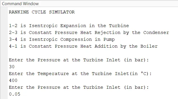
Input provided in command windows:
- Turbine Inlet temperature = 400° C
- Turbine Inlet Pressure = 30 bars
- Turbine Outlet Pressure = 0.05 bars = Condenser Inlet Pressure
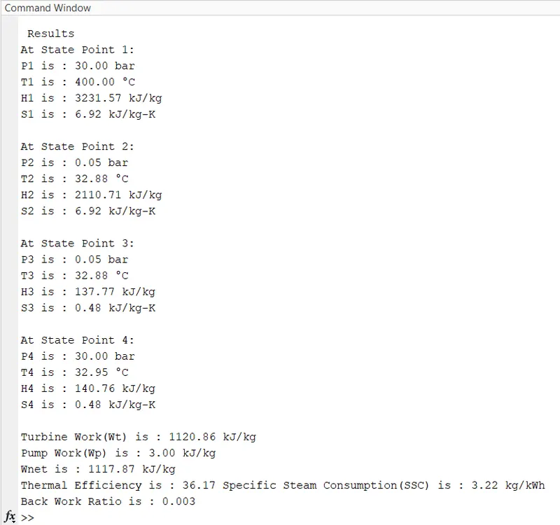
Result of Command Windows:
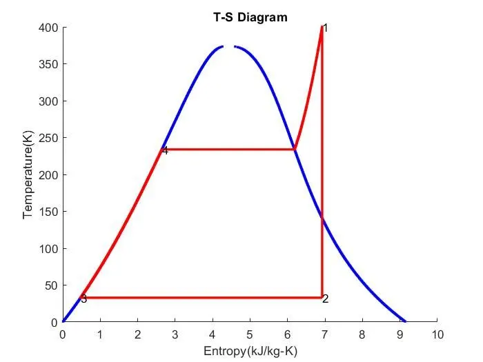
T-S Diagram:
H-S Diagram:
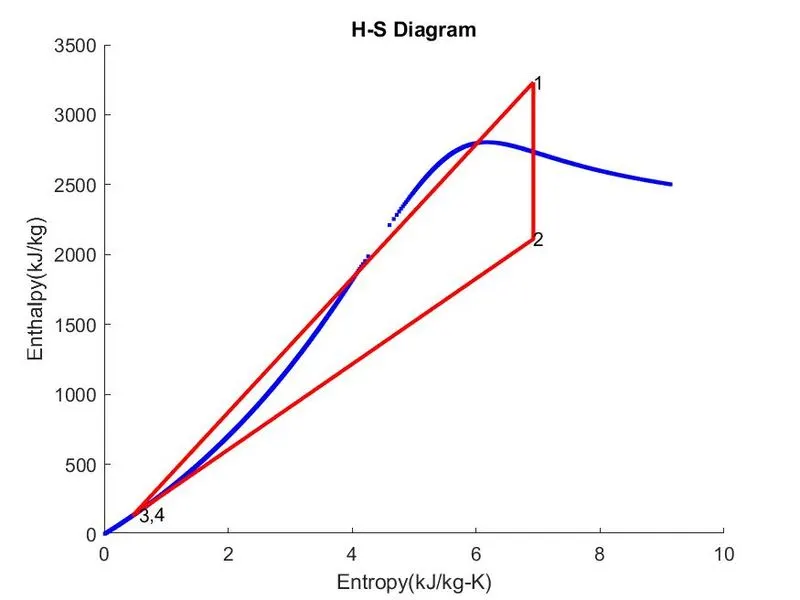
Here in both plots: The Blue Curve represents the Saturation Curve and the Red Curve represents the Rankine Cycle.
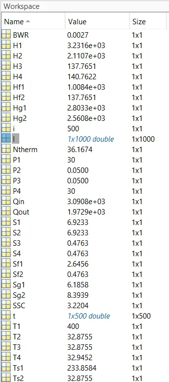
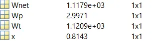
Workspace Values:
References:
https://mechanicalboost.com/rankine-cycle/#:~:text=The%20overall%20thermal%20efficiency%20of,make%201000%20MWe%20of%20electricity.