Week 7 State of charge estimation
Aim:- State Of Charge Estimation Using MATLAB Software
Objective:-
1.Simulate the 3 test cases from harness dashboard and write a detailed report on the results
2.What is coulomb counting? Refer to the above model and explain how BMS implements coulomb counting for SOC estimation ?
Introduction:-
State of charge (SoC)
The SOC of a battery pack is defined as the percentage of the RC (or RC divided by its rated capacity). In other words, SOC is the ratio between the saved energy in the battery and the total energy that can be saved in the battery. If the rated capacity is measured in coulombs or Ah, RC should also be estimated in the same units. In cases where the remaining or the rated energy content is estimated in watt-hours, SOC can be estimated based on the energy storage capability. The SOC provides the current state of the battery, and enables the battery to be safely charged and discharged at a level suitable for battery life enhancement.
It is common to estimate the SOC percentage using charge transfer in and out of the battery, and in this case typical coulomb-counting methods are used. In this case, we can use the rated capacity of the battery, Qrated, which is not a function of temperature or aging (since it is usually estimated at standard laboratory conditions at a controlled temperature). However, to accommodate the SOC variation with aging, it is necessary to use a different term, Qdischarge. This is defined as the maximum total electrical charge, expressed in Ah, that a battery can deliver from the fully charged state (SOC of 100%) to a fully discharged state (SOC of 0%) as indicated in Eq. (3.5),
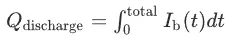
Then the SOC can be expressed using the ratio or percentage of the capacity that has been discharged relative to Qdischarge
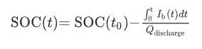
where Ib is the battery current.
In applications where energy transferred to and from the battery is considered, in Wh or kWh, one needs to use the integration of terminal voltage multiplied by the battery current, and this may be useful in applications where the true energy transferred between system elements is important. In applications such as EV, hybrid electric vehicles (HEV), and plug-in HEV (PHEV), since the engine capacities are measured in kW, battery pack SOC estimates are estimated based on the initial energy capacity E0(t) based on the relationship given in Eq. (3.7).

where E0(0) and Pi(t) are the initial energy capacity and the instantaneous power fed from the battery into the load, respectively. When Pi(t) is negative, the battery is charged from the external energy source. In this case, the system should have monitoring capability for both battery voltage and current. Kim and Cho (2011) and Ebbesen et al. (2012) provide some details on estimation of this useful parameter, and also some insight into dealing with practical inaccuracies in estimating the SOC and other useful parameters such as state of health (SOH).
Discription:-
1.Simulating the 3 test cases from harness dashboard and writing a detailed report on the results:-
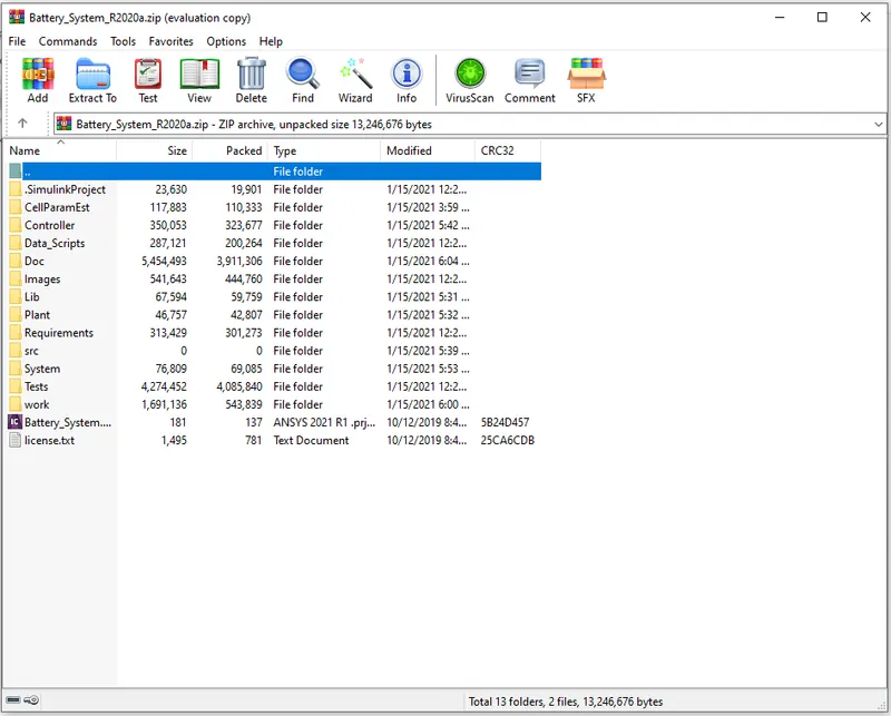
The file downloaded will be a zip file and it is extracted to a folder. The folder consist the files of both Battery_Systems_2020a and Battery_Systems_2019b.
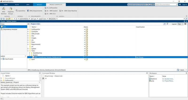
Now open the MATLAB software and open the model file ‘Closed loop BMS harness dashboard’ which is located in Tests-->System -->BMS_ClosedLoop_Harness_Dashboard.slx file.
After opening the file a pop-up dialog will open to install all the model related library files into the current folders and workspace
Blocks in the model:-
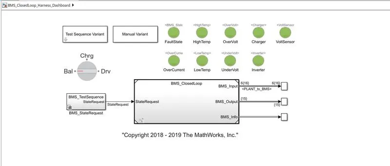
1)Dash board
- Manual variant (Selector)
- Test sequence variant (Selector)
- ‘BMS_Testsequence state request’ which is a Subsystem to provide state request commands.
- FaultState, HighTemp, OverVolt, Charger, VoltSensor, OverCurrent, LowTemp, UnderVolt and Inverter are Lamps which indicates three colors.
- a) Red color during fault conditions
- Green color during proper working conditions
- Rotating Switch is used for manual variant change while running
2)BMS_Closed loop
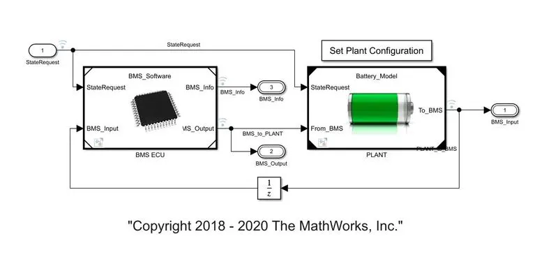
- It mainly consist of two subsystems and they are BMS ECU and PLANT.
- A closed loop is created by giving PLANT output as a feedback to the BMS ECU unit.
- The outputs obtained at set plant configuration are BMS_Output and BMS_Input.
Test case: 1
In test sequence variant select the choose Test case 1 and click on apply as shown in the figure below.
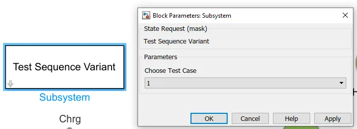
By selecting the test case 1 it will select the Testsequence 1 and remaining TestSequence2 and TestSequence3 will be comment out.
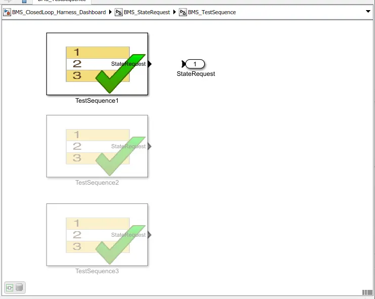
The Test case will be consisting of the following sequence operations as shown below.
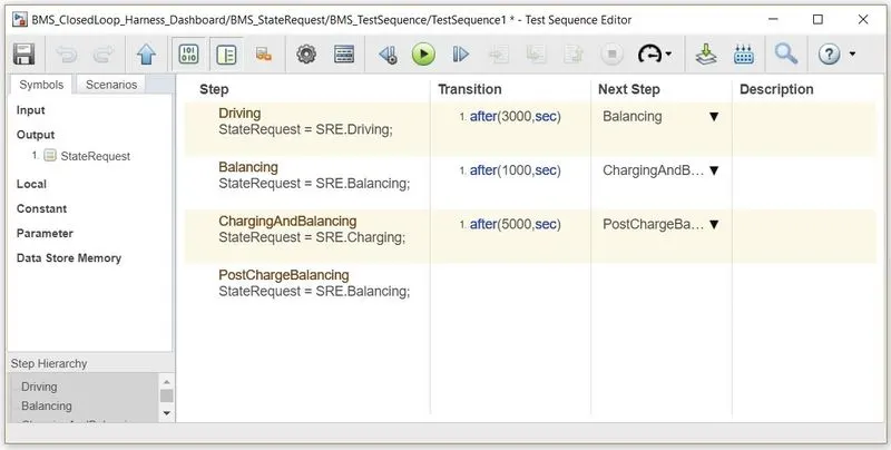
Here the driving will be done for 3000seconds then balancing will done for 1000seconds after that charging will be done in 5000 seconds. After completion of these three steps the post balancing operation will executed till the end of simulation period.
The simulation will be started by clicking the RUN button as shown in the figure below.
In the above figure all the lamps are indicating green color which means no faults during the operation of the test case-1.
TEST CASE-1 RESULTS:-
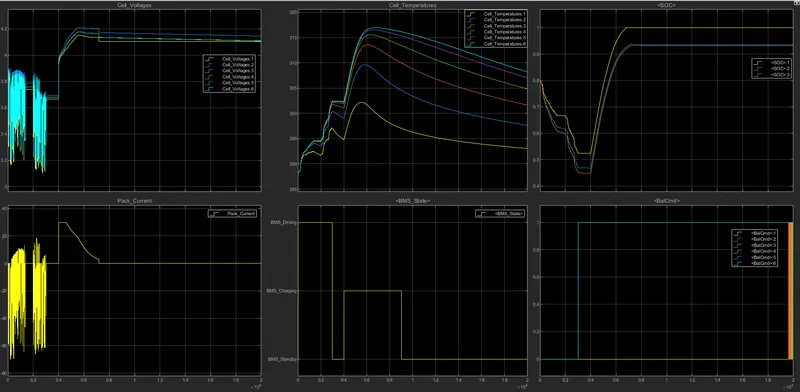
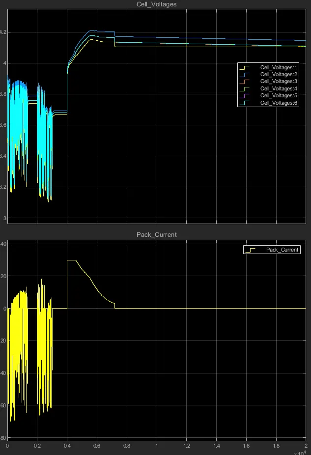
Cell voltage’s and pack current
- For the first 3000 seconds all the 6 cells are in drive mode where discharging occurs hence we observe the fluctuations in cell voltages which is varies between 3.1 to 3.9 volts.
- From 3000 to 4000 seconds is balancing where the module undergoes through standby mode where the voltage is maintained at a constant value of 3.7V.
- From 4000 seconds onwards the model undergoes through a charging mode. when the voltage is raised from 3.7V to 4 volts and the pack current is suddenly raised to 30Amp and when the cells voltage is increased from 4 to 4.2V the pack current starts to gradually decrease and attains a steady state value of 2.6A.
- At the end of 9000seconds we observe that all the cell voltages are balanced and with respect to cell 1 to a value of 4.1V as shown in the figure below.
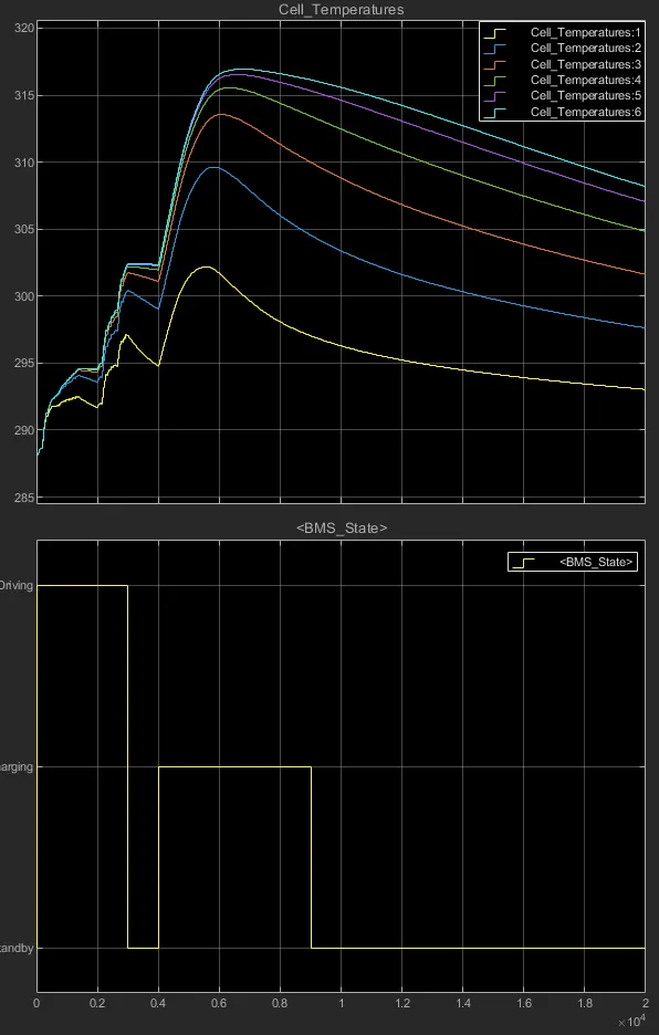
Cell temperatures:-
- From 0 to 3000 seconds the cell temperature starts to rise due to drive mode where the cells are continuously discharged. Here the temperature is raised from 288K to 302K.
- During standby mode which is from 3000 to 4000 seconds the cell temperatures are slightly reduced as there will be no current flow.
- After 4000seconds the temperature starts to increase exponentially upto a constant current region and starts to reduce as the current flow start to reduce and become a constant value from 7000seconds onwards.
- From the below figure we observe the maximum temperature rise occured on cell 6 which is 317K while the cell 1 temperature raised upto 302K.
BMS State:-
- From 0 to 3000 seconds the battery module in drive mode which is discharging.
- From 3000 to 4000 seconds the battery module is in balancing standby mode as shown from result plot.
- After 4000 seconds upto 9000 seconds the battery module in charging and balancing mode.
- After 9000 seconds only post charge balancing operates upto end of simulation.
SOC (STATE OF CHARGE):-
- From the below graph we observe that initially the SOC of a battery module is 80%.
- Yellow color plot represents SOC estimation by coloumb counting technique.
- Blue color plot represents SOC estimation by Unscented Kalman filter technique.
- Red color plot represents SOC estimation by Extended Kalman filter technique.
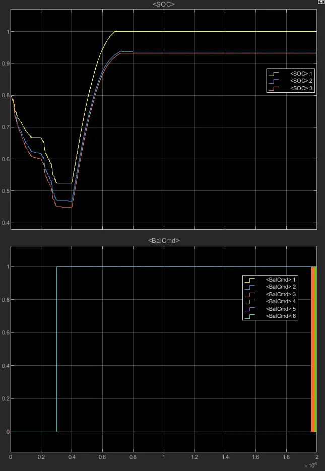
From 0 to 3000seconds SOC decreased from 80% to 45% during the Drive mode and from 3000 to 4000 Seconds the SOC value remains constant due to cell balancing in Standby mode after that SOC starts to increase till 94% due to charging mode from 4000 to 9000 seconds.
Balancing cells:-
from 0 to 3000 seconds is drive mode hence balancing is not performed and the values of all cells are at zero. After the 3000 seconds the balancing of cell 2 & cell 6 are done since there voltage is higher than all the other cell voltages and in the end of simulation all the cell voltages are balanced by a common value which is one.
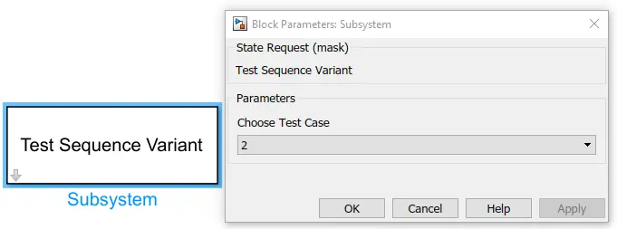
Test case 2:-
Now we have to select the test case2 by clicking on test sequence varient dialog box as shown below.
By selecting the test case2 the TestSequence2 is selected and remaining will be comment out as shown in the figure below.
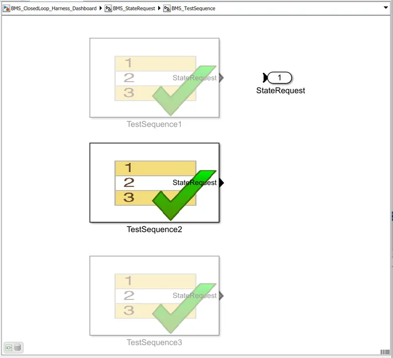
The test case consist of a drive mode for a duration of 10,000 seconds and after that charging occurs till the end of simulation.
The results of test case 2 are shown below graphs.
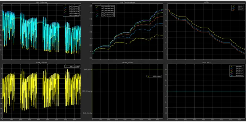
Cell Voltages and pack Current:-
- The cell voltage is varied between 3.05V to 3.9V.
- The pack current discharges upto 70Amps.
Cell Temperature:-
- from cell temperature graph we observe that the cell 6 is having the maximum temperature variation which is 288K to 322.5K, while the cell 1 is having the minimum variation in temperature which is 288K to 302.5K
- The temperature difference between cell 1 and cell 6 is 20°C.
BMS_State:-
- From BMS_state graph we observe that the entire test sequence is in drive mode from 0 to 9000 seconds.
SOC :-
- The SOC was decreased from 80% to 0% during the time 0 to 9000 seconds since the test sequence was operated in drive mode.we observe constant SOC during certain particular intervals due to standby mode.
Balancing:-
- From 0 to 9000 seconds the balancing of cells was noto performed due to drive mode.
Test case 3:-
Now we have to select the test case3 by clicking on test sequence varient dialog box as shown below.
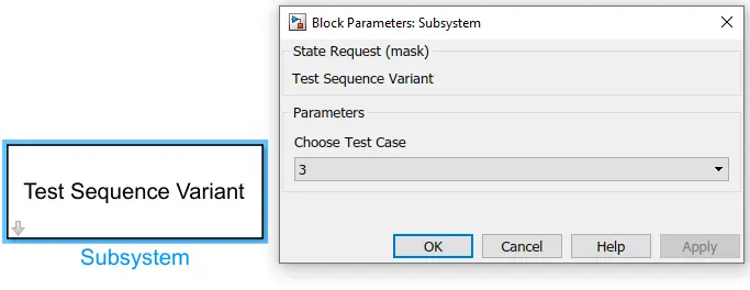
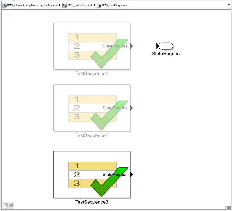
By selecting the test case 3 the TestSequence3 is selected and remaining will be comment out as shown in the figure below.
The results of test case 3 are shown below graphs.
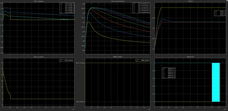
BMS_State:-
- From BMS_state graph we observe that the entire test sequence is in charging mode from 0 to 2000 seconds.
Cell Voltages and pack Current:-
- The battery pack will take large amount of pack current in the starting since the SOC is 80% after 2000 seconds the SOC will be 100% hence the pack current after 2000 seconds is zero ampere.Similarly, cell voltages are also reached to a constant value after 2000seconds.
Cell Temperature:-
- The cell temperature were continously rising till all the 6 cells are fully charged which is upto 2000 seconds. after that temperaure starts to decrease gradually.
SOC :-
- The SOC of the battery pack in the begining was 80% and it is increased to 100% due to charging mode in 2000 seconds.
Balancing:-
- cell 2 & cell 6 are balanced from the begining of the simulation with respect to cell 1 and during the end of simulation all the cell will undergo balancing.
2) What is coulomb counting? Refer to the above model and explain how BMS implements coulomb counting for SOC estimation ?
Coulomb counting is a technique used to track the State of Charge of a battery pack. It works by integrating the active flowing current (measured in amps) over time to derive the total sum of energy entering or leaving the battery pack.
Coulomb counting
To determine available capacity, coulomb counting relies on the integration of the current drawn from and supplied to a battery over time,
as given by
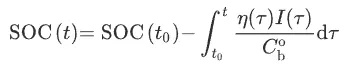
where I is the current and η is the efficiency during charge and discharge operations. Coulomb counting is advantageous in terms of a simple structure and its ease of implementation. However, some problems make it difficult to accurately estimate battery SOC by coulomb counting. Because battery capacity and efficiency are significantly influenced by operating temperature and current direction, these factors should be considered to correct for battery SOC. Sensor accuracy is also important because accumulated errors can lead to a drift in the estimated battery SOC. Furthermore, one of the main problems in coulomb counting is that it is necessary to calibrate the initial battery SOC. In several applications, the initialization involves rest and the initial SOC is estimated based on the voltage inversion method.
coulomb counting for SOC estimation in BMS Model :-
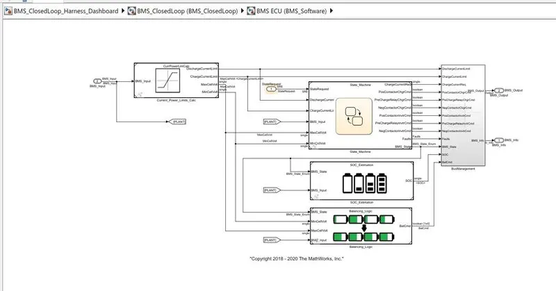
In order to find the coulomb counting in BMS model we have to double click on SOC_Estimation and then double click on coulomb counting which is shown in the below figures.
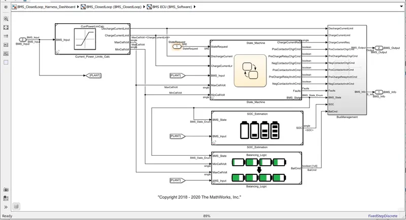
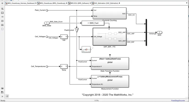
the below figure represents the coulomb counting Simulink model.
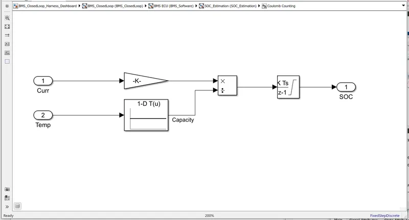
It basically consists of four blocks, they are
a) gain
b)1-D Lookup Table
c)divide
d)Discrete-Time Integrator
Explaination:-
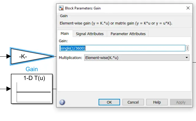
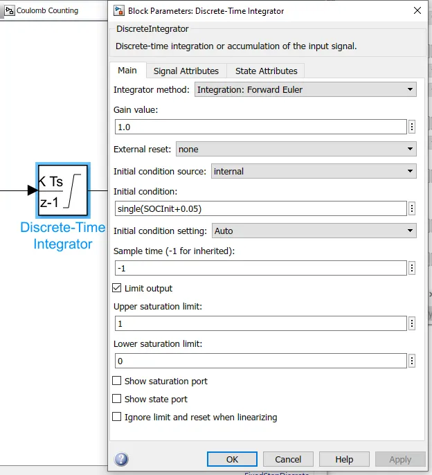
The discharge current which is coming from the is given to gain block with a value of 1/3600 to convert current into ampere Hour (Ahr). The value Ahr is divided with capacity due to temperature change. The obtained value is then integrated with a gain value of 1 and sample time of -1. Since we are using Discrete- Time Integrator with a saturation limit from 0 to 1. The output obtained from Discrete-Time Integrator will be SOC from 0 to 100%.
Conclusion:- All the three test cases and coloumb counting were properly explained by using a BMS_ClosedLoop_Harness_Dashboard model in MATLAB 2020a Software.