Project

Aim: - To Study The System-Level Simulation Of An All-Terrain Vehicle Under Different Conditions.

Objective: - Carry out a system-level simulation of an all-terrain vehicle. Prepare a technical report explaining the model properties & comments on the results.

Introduction To All-Terrain Vehicle (ATV):-

An all-terrain vehicle (ATV), also known as a light utility vehicle (LUV), a quad bike, or simply a quad, as defined by the American National Standards Institute (ANSI); is a vehicle that travels on low-pressure tires, with a seat that is straddled by the operator, along with handlebars for steering control. As the name implies, it is designed to handle a wider variety of terrain than most other vehicles. Although it is a street-legal vehicle in some countries, it is not street-legal within most states, territories, and provinces of Australia, the United States or Canada.

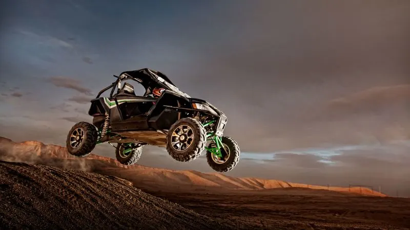
Figure-1.1

• Transmission in vehicles is basically transmitting the power from engine to the wheels. There are three types of transmission in vehicles.

1. Manual transmission
2. Semi-automatic transmission
3. Automatic transmission

1. Manual transmission

A manual transmission (also known as a manual gearbox; abbreviated as MT, and sometimes called a standard transmission in the US) is a multi-speed motor vehicle transmission system, where gear changes require the driver to manually select the gears by operating a gear stick and clutch (which is usually a foot pedal for cars, or a hand lever for motorcycles).

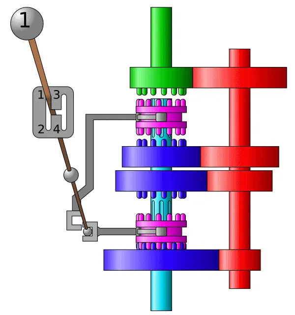
Figure-1.2

2. Semi-automatic transmission

Semi-automatic transmission denotes a multi-speed motor vehicle transmission where part of its operation is automated (typically the clutch actuation), but the driver's input is still required to start (i.e., launch the vehicle) from a standstill and to manually change gears.

3. Automatic transmission

An automatic transmission (sometimes abbreviated to auto or AT) is multi-speed transmission used in motor vehicles that does not require any driver input to change gears under normal driving conditions.

The most common type of automatic transmission is the hydraulic automatic, which uses a planetary gear set, hydraulic controls, and a torque convertor. Other types of automatic transmissions include continuously variable transmissions (CVT), automated manual transmissions (AMT), and dual-clutch transmissions (DCT).

3.1. Continuous variable transmission

• A continuously variable transmission(CVT) is an automatic transmission that can change seamlessly through a continuous range of gear ratios. This contrasts with other transmissions that provide a limited number of gear ratios in fixed steps. The flexibility of a CVT with suitable control may allow the engine to operate at a constant RPM while the vehicle moves at varying speeds.

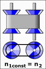
Figure-1.3

Software Used: - Matlab and Simulink

Simscape Model of ATV:-

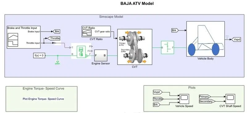
Figure 1.4

COMPONENTS PRESENT IN SIMSCAPE MODEL:-

1. INPUT BLOCKS a) Throttle b) Brake c) Cvt Gear Ratio
2. GENERIC ENGINE a)Engine Sensor b)Simple Gear
3. CVT a)Variable Transmission b) Inertia of rotating parts
4. VEHICLE BODY a) Physical Body b) Tire c) Shoe Brake

INPUT TO THE SYSTEM:-

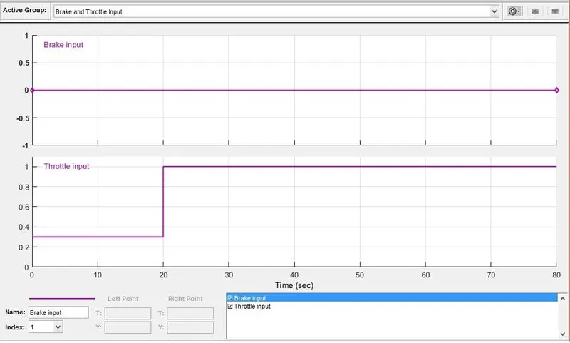
Figure 1.5

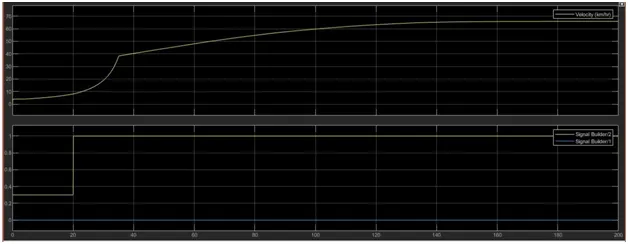
The inputs are given from the signal builder as shown in the above figure 1.5. Here we are using both brake and throttle as inputs, in which brake input remains constant at a zero and throttle input is varied from 0.3 to 1 at 20^th second. The generated signal is given as an input to generic engine.

Generic Engine:-

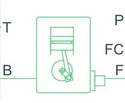
Figure 1.6

It represents system level model of spark ignition and diesel engines suitable for the use at initial stage of modeling when only basic parameters are available. An optional idle speed controller is included.

The throttle input signal T lies between zero and one and specifies the torque demanded from the engine as a fraction of the maximum possible torque. If the engine speed falls below the Stall speed, the engine torque is blended to zero. If the engine speed exceeds the Maximum speed, the simulation stops and issues an error message.

Connections F and B are mechanical rotational conserving ports associated with the engine crankshaft and engine block, respectively. Connections P and FC are physical signal output ports through which engine power and fuel consumption rate are reported.

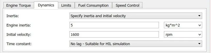
Engine Parameters:-

Engine Sensor:-

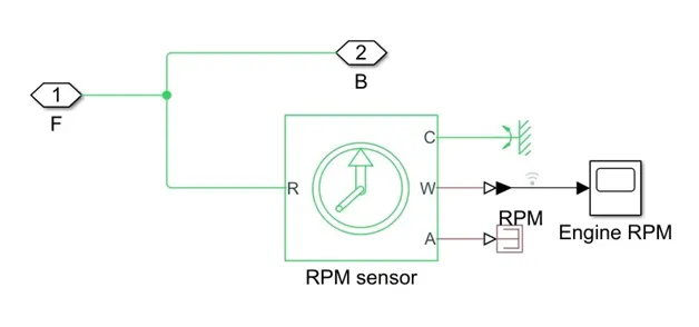
Figure 1.7

The block represents an ideal mechanical rotational motion sensor which converts variables measured between two mechanical rotational nodes into a control signal proportional to angular velocity or angle. Since it is an ideal sensor, It does not account for friction, Inertia, Delays, Energy consumption and so on.

The connections R and C are mechanical rotational conserving ports and connections W and A are physical signal output ports for velocity and angular displacement.

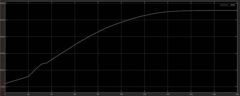
Figure 1.8

From the above graph it is clear that the RPM gradually increased from 1620 to 3750 in 0 to 140 seconds of time duration.

Engine torque v/s speed graph:-

The data was extracted from actual all terrain vehicle. So, that our model provides us real time

Analysis.

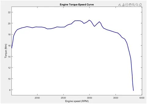
Figure 1.9

Continuously Variable Transmission (CVT):-

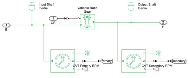
Figure 1.10

• The figure consists of input shaft inertia and output shaft inertia which represents the primary and secondary pulley.
• The variable gear ratio block is used to model a continuously variable transmission.

1. It represents a variable ratio gearbox such as implemented by a mechanical belt CVT or hydraulic transmissions. The physical signal input R defines the ratio of input to output angular shaft velocities.
2. Connection B (base) and F (follower) are mechanical rotational conserving ports. Specify the relation between base and follower rotation directions with the Output SHAFT rotates parameter.

CVT Gear Ratio Given As Input To CVT:-

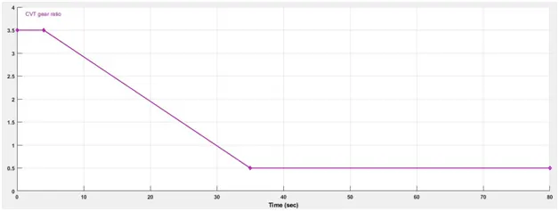
Figure 1.11

• VEHICLE BODY DIAGRAM:-

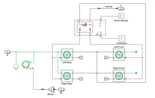
Figure 1.12

The vehicle body mainly consists of tires, Double Shoe Brake, inertia block which are connected to main vehicle body.

1.Main Vehicle Body:-

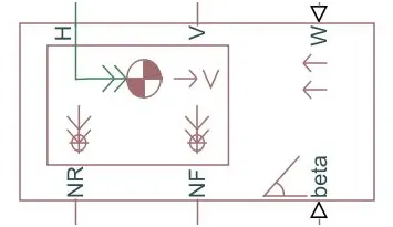
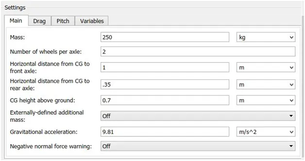
Figure 1.13

It Represents a two-axle vehicle body in longitudinal motion. The block accounts for body mass, aerodynamic drag, road incline, and weight distribution between axles due to acceleration and road profile. The vehicle can have the same or a different number of wheels on each axle. Optionally include pitch and suspension dynamics or additional variable mass and inertia. The vehicle does not move vertically relative to the ground.

Connection H is the mechanical translational conserving port associated with the horizontal motion of the vehicle body. The resulting traction motion developed by tires should be connected to this port. Connections V, NF, and NR are physical signal output ports for vehicle velocity and front and rear normal wheel forces, respectively. Wheel forces are considered positive if acting downwards. Connections W and beta are physical signal input ports corresponding to headwind speed and road inclination angle, respectively. If variable mass is modeled, the physical signal input ports CG and M are exposed. CG accepts a two- element vector representing the x and y distance offsets from vehicle CG to additional load mass CG. M represents the additional mass. If both variable mass and pitch dynamics are included, the physical signal port J accepts the inertia of the additional mass about its own CG.

2.Tire (magic formula):-

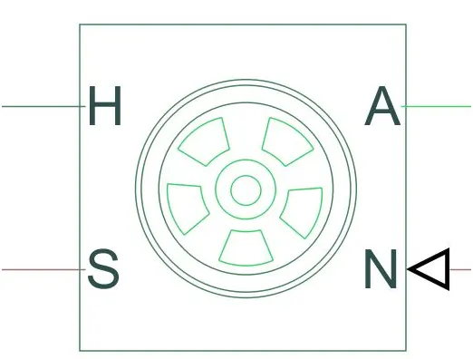
Figure 1.14

Represents the longitudinal behavior of a highway tire characterized by the tire magic formula. The block is built from tire-road interaction (magic formula) and Simscape foundation library wheel and axle blocks. Optionally, the effects of tire inertia, stiffness, and damping can be included.

Connection A is the mechanical rotational conserving port for the wheel axle. Connection H is the mechanical translational conserving port for the wheel hub through which the thrust developed by the tire is applied to the vehicle. Connection N is a physical signal input port that applies the normal force acting on the tire. The force is considered positive if it acts downwards. Connection S is a physical signal output port that reports the tire slip. Optionally expose physical signal port M by setting parameterize by to physical signal magic formula coefficients. Physical signal port M accepts a four element vector corresponding to the b, c, d, and e magic formula coefficients.

3.Double Shoe Brake:-

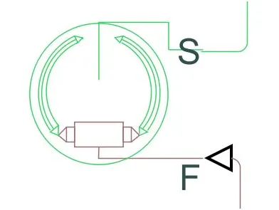
Figure 1.15

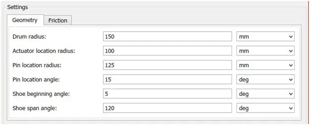
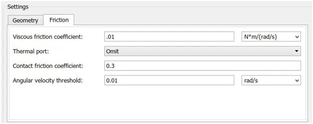
It represents a brake arranged as two pivoted rigid shoes symmetrically installed inside or outside a drum and operated by one actuator. The actuator force causes the shoes to exert a friction torque on a shaft connected to the drum.

Connection S is a conserving rotational terminal associated with the drum shaft. Connection F is a physical signal port representing the force input to the actuator. Positive force creates friction torque that resists shaft rotation. Optionally include thermal effects and expose thermal conserving port H by setting Thermal port to Model.

4.Inertia:-

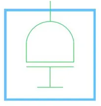
Figure 1.16

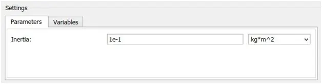
This block represents ideal mechanical rotational inertia. The settings are given below

Output Graph:-

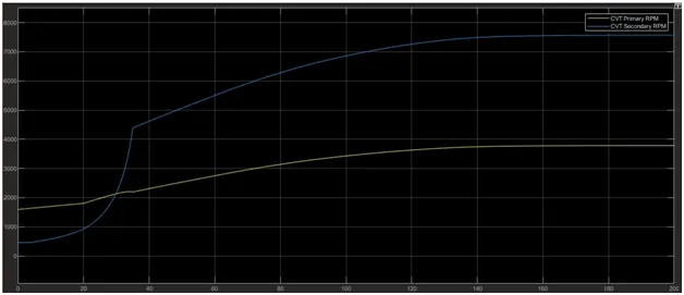
From the graph, It is clear that at 30sec time duration the RPM of secondary goes higher than the primary and difference in rpm is more than 3500 RPM. Hence, the ATV velocity is also increases.

Baja ATV Dashboard Model:-

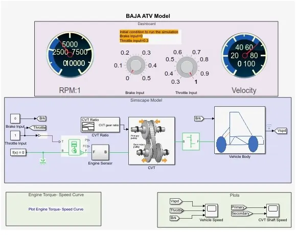
Figure 1.17

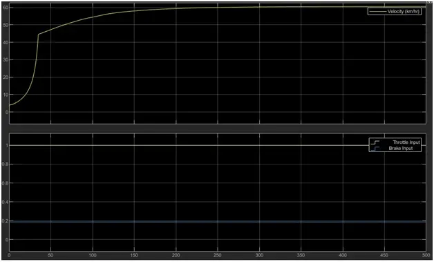
The dashboard model is similar to the CVT model with signal builder is replaced with control knobs. With the help of throttle input and brake input knobs the output can be obtained for infinite time duration and dashboard helps to see RPM and velocity variations directly on the display.

Output Graph:-

Baja ATV Closed Loop Model:-

This model is also similar to the Baja ATV model in figure 1.4 but, In the closed loop model the output of vehicle body is given as feedback to the CVT which is shown in figure 1.18, The CVT gear ratio is obtained from lookup table which is shown in fig 1.20

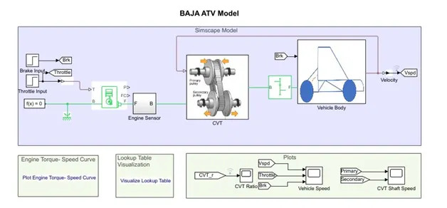
Figure 1.18

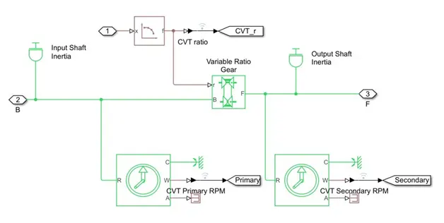
Figure 1.19

Lookup table visualization:-

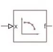
Figure 1.20

This block represents a physical system converter whose input- output relation is specified by a lookup table. The table grid must be in a strict ascending or descending order, but spacing can be non uniform.

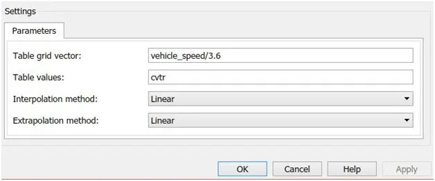
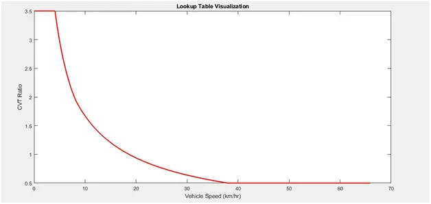
Figure 1.20

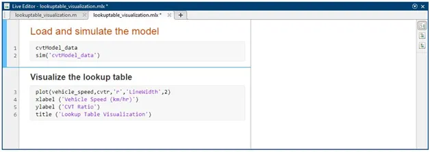
Matlab Program Inserted In The Workspace:-

Result:-

Baja All terrain vehicle can be simulated either using feedback, signal generator and dashboards, the vehicle velocity and secondary RPM outputs will remain same for the same specifications.